Assembly Sequence Planning for Motion Planning

JOURNAL OF LATEX CLASS FILES, VOL. X, NO. X, XXXX 2016

1

Assembly Sequence Planning for Motion Planning

arXiv:1609.03108v1 [cs.RO] 11 Sep 2016

Weiwei Wan, Member, IEEE, Kensuke Harada, Member, IEEE, Kazuyuki Nagata, Member, IEEE

Abstract—This paper develops a planner to find an optimal assembly sequence to assemble several objects. The input to the planner is the mesh models of the objects, the relative poses between the objects in the assembly, and the final pose of the assembly. The output is an optimal assembly sequence, namely (1) in which order should one assemble the objects, (2) from which directions should the objects be dropped, and (3) candidate grasps of each object. The proposed planner finds the optimal solution by automatically permuting, evaluating, and searching the possible assembly sequences considering stability, graspability, and assemblability qualities. It is expected to guide robots to do assembly using translational motion. The output provides initial and goal configurations to motion planning algorithms. It is ready to be used by robots and is demonstrated using several simulations and real-world executions. Index Terms—Grasp Planning, Manipulation Planning, Object Reorientation

the three capacitors first and then attach the switch button on top of it. Fig.1(c.1-4) illustrates this optimal solution. In contrast, a bad assembly sequence is shown in Fig.1(a.1-4) where after inserting two surrounding capacitors in (a.2) and (a.3), it is difficult to find an collision-free grasp to insert the third capacitor into the middle slot (see (a.4)). Another bad assembly sequence is shown in Fig.1(b) where two capacitors are inserted in (b.1) and (b.2), and the switch button is attached in (b.3). It is impossible to insert the third capacitor in (b.4). Human beings could easily find inserting the third capacitor in (a.4) and (b.4) are bad choices since the surrounding capacitors or the switch button would block the motion. However, it is a non-trivial problem to robots. Traditionally methods used in robotic assembly are that skilled human technicians teach robots the assembly orders and directions, which makes robotic manufacturing less robotic.

I. Introduction

A

SSEMBLY planning implies a wide range of concepts. It includes task and symbolic planning in the high level, motion planning in the middle level, and force and torque control in the low level. In this paper, we focus on the high-level assembly sequence planning problem and develop a planner that could automatically find an optimal assembly sequence which is ready to be used by robots for motion planning. The input to the planner includes • Mesh model of a robotic hand. • Mesh models of objects. • Relative poses between objects in the assembly. • Goal pose of the assembly. The output includes • Assembly order: Which objects to assemble first. • Assembly direction: How to drop or insert objects. • Accessible grasps: How to grasp objects during assembly. The proposed planner finds the optimal solution by automatically permuting, evaluating, and searching the possible assembly sequences considering stability, graspability, and assemblability qualities. It is expected to guide robots to do assembly using translational motion. The planner is born for motion planning as the output provides initial and goal configurations for robots to carry out motion planning algorithms. The study is motivated by an assembly task in real world where the goal is to assemble a switch shown in Fig1(c.4). The switch is composed of five parts shown in Fig.1(a.1). A robot needs to insert three capacitors into a base and attach a switch button on top of it. An optimal sequence to finish this task is, as was described in the last sentence, to insert Weiwei Wan, Kensuke Harada, and Kazuyuki Nagata are with National Institute of Advanced Industrial Science and Technology (AIST), Japan. Kensuke Harada is also affiliated with Osaka University, Japan.

[email protected]

Fig. 1: Assembly a switch. (a) and (b) are two bad choices due to collision between grippers and surrounding capacitors or collision between the active capacitor and the finished part. (c) is an optimal sequence. The planner challenges the non-trivial problem by performing assembly sequence planning. It finds the optimal assembly sequence by automatically permuting, evaluating, and searching the objects. First, it permutes the objects and lists all assembly orders. Each assembly order includes a sequence of objects that should be assembled sequentially. Then, for each assembly order, the planner manipulate the object in the sequence one by one and evaluate the stability and the graspability of each manipulated object. Meanwhile, it checks if the manipulated object can be assembled, computes its optimal assembly directions considering the normals of contact surfaces, and evaluates the assemblability (tolerance to errors) of the optimal assembly directions. Using these permuting, evaluating, and searching steps, the approach is able to find some optimal assembly orders and directions that are (1) stable after assembling each manipulated object, (2) have lots of accessible grasps and are flexible to the kinematic


constraints of robots, and (3) robust to assembly errors. Comparing with contemporary studies, our main contribution is we do everything automatically in 3D workspace, considering not only stability and assemblability, but also graspability. The benefit is the planned results could be seamlessly used by robot motion planners: The accessible grasps work as initial and goal configurations for robot end-effectors; The assembly directions work as motion primitives. The assembly planner is born for motion planning. The experimental section of this paper not only presents and analyzes the results of the assembly planner, but also includes some real-world executions that use integrated assembly sequence planning and motion planning. II. Related Work Early studies in assembly planning are symbolic reasoning systems [1] [2] and use given contact and assembly constraints to do decision search. For example, Mello, et al. [3] is a representative one which used logical expressions to defined the assemblies and used a relation model graph to generate assembly sequences. It considered geometric-feasibility, mechanicalfeasibility, and stability during searching. Sanderson [4] performed robust symbolic assembly planning by considering the clearance between contacting objects. It is the first work which used the keyword “assemblability”. Reference [5] is a more recent work that used symbolic reasoning. The work is quite practical as it included some real-world executions. Knepper, et al. [6] also ran some real-world executions. The study not only used symbolic planning to find assembly sequences, but also used geometric analysis to infer how to attach pins to holes. In another paper [7], Knepper further formulated assembly sequence planning as a task allocation problem and proposed a method to plan assembly sequences that could be done in parallel. Comparing with symbolic assembly planning, geometric reasoning systems generate assembly sequences by automatically discovering contact and assembly constraints. The earliest geometric reasoning-based assembly planning systems we could find is [8]. The work used geometric constraints to build a disassembly tree and employed the tree to find an assembly sequence for a restricted class of problems. Another representative study is reference [9] which used the geometric constraints to build a Non-Directional Blocking Graph (NDBG) and employed the graph to reason about assembly sequences. Romeny, et al. [10] extended the NDBG to 3D assembly by using a sphere of directions of motion. One region on the sphere was associated with one DBG and the sphere and the DBGs together added up to the NDBG. Assembly sequences were planned by analyzing the sphere and its associated DBGs. Ikeuchi, et al. [11] used constraint Gaussian spheres to represent the contact constraints between mesh models, and planned assembly sequences by considering the constraint spheres at each contact. Thomas, et al. [12] represented the assembled objects using stereographical projections and figured out a different way to denote separability. The stereographical projection essentially shares the same idea with constraint spheres except that it could handle complex

2

polyhedrons quickly. A good summary of the studies that plan assembly sequences using geometric reasoning before 2013 could be found in [13]. The early assembly planning systems only considered a single constraint model (mostly geometric constraints). More recent work considers a mixed model of constraints. For example, Agrawala, et al. [14] used NDBG to generate assembly sequence and used visibility constraints to find an view-friendly assembly sequence which could be drawn on a paper document as assembly instructions. The constraint model is a mixture of geometric constraints and visibility constraints. OstrovskyBerman, et al. [15] discussed the tolerance of different contact types and used them to optimize assembly sequence planning. The tolerance is similar to the concept of “assemblability” in [4], and the constraint is a mixture of geometric constraints and uncertainty constraints. Schwarzer, et al. [16] additionally considered m-handed assembly which allowed m objects to be disassembled simultaneously. Wei [17] applied the automatic assembly sequence generation to ship building by considering the sizes, positions, and materials of the objects. Dobashi, et al. [18] additionally considered the collision-free grasps between manipulated objects and the assembled objects during assembling, although the assembly sequence is pre-defined manually considering these constraints. McEvoy, et al. [19] considered both stability and geometric constraints in planning the assembly sequences of truss structures. A real-world execution is included in their paper. Dogar, et al. [20] used several mobile robots to assemble a chair. The constraints between robots, between robot grippers and the assembled objects, and between manipulated object and assembled objects, are considered during the assembly. The paper also includes a realworld execution. Ghandi, et al. [21] made a good summary of the studies dealing various constraints before 2015. In this paper, we perform assembly sequence planning considering statics constraints of the assembled part (stability), quasistatic constraints between grippers and manipulated objects and geometric constraints between grippers and surrounding objects (graspability), and geometric constraints between the manipulated object and the finished part (assemblability). We evaluate the quality of stability, grasplability, and assemblability to find an optimal sequence for translational assembly. We assume the objects are 3D polyhedron, the assembly motion are translational, and a single gripper is used at one time. Comparing with previous work, we not only present planners which consider a mixed model of the constraints that directly relate to robot motion planning, but also demonstrate the pragmatic flavor of our system using the real-world executions of several exemplary tasks. III. Overview of the Approach We present the algorithmic part of this paper using soma cube as an example to promote clarity. Soma cube is a solid dissection puzzle invented in 1933. Three blocks, an z-shape block, a t-shape block, and a tri-shape block of the soma cube puzzle are used to assemble a given structure (see Fig.2). The input to the planner is the mesh models of the three objects, their relative poses, and the final pose of the assembly. The


3

output is the assembly order, the assembly directions, and the candidate grasps of each object. The input and output are shown in the frameboxes of Fig.2 (The candidate grasps are not shown in the figure).

Fig. 3: The algorithmic flow of the proposed approach. Fig. 2: The input and output of the planner. The algorithmic flow of the proposed approach is shown in Fig.3. The input includes: (1) The mesh model of the robotic hand; (2) The mesh models of the objects; (3) The relative poses between the objects in the assembled structure; (4) The final pose of the assembly. First, using the number of objects, the planner computes all possible permutations in the permutation toolbox. For each permutation, the approach evaluates its stability, graspability, and assemblability qualities. The stability quality is evaluated by computing the relationship between pcom (center of mass) and the boundary of supporting area. It is denoted by S in the figure. The graspaibility quality is evaluated by computing the number force-closure and collision-free grasps. Using the mesh model of the robotic hand and the mesh models of the objects, the planner computes the possible hand configurations to grasp the object in the “force-closure grasps” box without considering collisions with other objects. The “graspability quality” box removes the force-closure grasps that collide with the finished part and counts the number of remaining grasps as the quality of graspability. Graspability is denoted by G in Fig.3. The assemblability quality is evaluated using the normals of the contact faces between the manipulated object and the finished part. The process is done in the “Assemblability Quality” box. If the current permutation is assemblable, the planner uses the direction that has largest clearance from all contact normal as the assembly direction, and sets its quality A considering the size of the clearance. After evaluating the qualities, the approach compares the G, S, and A of each permutation, selects the permutation that has max(min(G) · min(S) · min(A)) as the optimal assembly order, and selects its correspondent assembly directions as the optimal assembly direction. The details of this expression will be explained in next section. IV. Implementation Details A. Permutation Given the total number of the objects to be assembled, permutation permutes object IDs and lists all the possible assembly orders without considering any constraints. n objects lead to Pnn = n! permuted orders. There are three cubes in the example shown in Fig.2 and therefore the number of permuted orders is 3! = 6. Consider three objects with ID “Z”, “T”, “Tri” (Fig.2), the output of the permutation is Tri ← Z ← T,

Tri ← T ← Z, Z ← Tri ← T, Z ← T ← Tri, T ← Z ← Tri, T ← Tri ← Z, and each element, for example T ← Tri ← Z, indicates a potential assembly order which first assembles object Tri to T, and then assembles object Z to the complex of T and Tri. For a subsequence T ← Tri, T is called the base object, Tri called the manipulated object. When assembling Z to the complex of T and Tri, Z is the manipulated object. (T, Tri) is the base. The reason permutation is used instead of AND/OR graph is we not only consider assembling two objects using “AND”, but also consider the order of the assembly, namely which one is the base and which one is the manipulated object. (Note: Some potential assembly orders may be infeasible. They will be removed progressively when computing the qualities.) B. Stability Stability is evaluated sequentially for each object in each potential order. The first step is check if the assembled part is stable after assembling the manipulated object following a given potential order. The stability qualities of unstable objects will be set to 0. Deciding whether an object is stable can be performed by projecting its center of mass pcom and supporting area to a horizontal plane, and checking if the projected pcom is inside the convex hull of the projected area. The object is not stable the projected pcom is outside the hull. The green shadow point and the dash boundaries in Fig.4(a) and (b.3) are the projections of pcom and the supporting area. The two manipulated objects are both stable. If the manipulated object is stable, the next step is to evaluate its stability quality. This is implemented by finding the nearest point pb on the convex boundary of its supporting area (which might be from both the base and the environment) to the manipulated object’s pcom and compute the angle between → the vector − p−b−p−− com and the horizontal plane. A smaller angle avoids large disturbance torques, indicating higher stability. Take T ← Tri ← Z, for example. The first step of stability evaluation is to compute the stability of T. Since the final configuration of the assembly is a given parameter, the poses of T, Tri, and Z are pre-known. The first step therefore equals to evaluating the stability of T at a given pose. Fig.4(a) shows this simple case and the angle that indicates the quality. The second step is to evaluate the stability of object Tri. Computing → the angle between − p−b−p−− com and the horizontal plane becomes complicated since the supporting area could be from both the


4

table surface and the surface of T. We solve this problem by using the 3D boundary shown in Fig.4(b) and (b.1, b.3, b.4).

Fig. 4: Computing the stability of the manipulated object by → measuring the angle between − p−b−p−− com and a horizontal plane. (a) shows the first step. The red dash line shows the vector − → p−b−p−− com . The grey square indicates a horizontal plane. (b) shows the second step where the supporting boundary is 3D. The third step evaluates the stability of object Z. Like the second object, the third object could also be supported by both the table surface and the surfaces of the finished part. We use the same technique as Tri to compute its stability quality. The result of the stability evaluation is a triple s=(s1 , s2 , s3 ) where each element indicates the stability quality of each object when doing assembly following the potential order. The stability qualities of all permuted orders form a column of triples named S where     s1   s11  s   s S =  2  =  21 . . .  . . . s6 s61

s12 s22 s62

 s13   s23    s63

(1)

C. Graspability For a potential order computed by (1), its graspability is computed by sequentially counting the force-closure and collision-free grasps of each object. The process is the same as a precedent work where we compute the force-closure grasps of all candidate objects (Section 4 of [22]). During assembly planning, we remove the collided grasps from the precomputed force-closure set and count the number of remaining grasps (known as accessible grasps) as the graspability. An example is shown in Fig.5. For the first object in the potential order, we only check the collision between the hand and the table surface. For the second and third objects, we check both the collision between the hand and the table, and the collision between the hand and the finished part. The output of graspability evaluation for a potential order is a triple g=(g1 , g2 , g3 ) where each element indicates the graspability quality of each object when doing assembly following the order. The graspability qualities of all permuted orders form a column of triples named G where     g1  g11  g  g G =  2  =  21 . . .  . . . g6 g61

g12 g22 g62

 g13   g23    g63

(2)

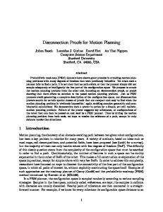
Fig. 5: Computing the graspability of the manipulated object by counting the number of accessible grasps. (a) Sample the surface of the object model. (b.1) For each pair of the sample, find force-closure grasps. (b.2) One grasp is represented by a segment plus a coordinate attached to its end. (c.1) All grasps after rotating and collision checking with the object itself and the table surface. (c.2) Simplified representation (coordinates are not shown). If this object is the first object, the number of segments in (c.2) will be its graspability. If the object is not the first one ((c.3)), remove the grasps that collide with the finished part (grey object in (c.3)) and count the remaining grasps as the graspability. D. Assembly directions and assemblability The assembly directions and assemblability of a potential assembly order are computed and evaluated using the normals of the contact faces between the newly added object and the finished part. In theory, we are using the constraint spheres shown in the second row of Fig.6. In implementation, we compute the convex hull of the contact normals and perform piece-wise analysis considering the types of the convex hull and the position of the origin with respect to the hull (third row of Fig.6). For each object, we compute its optimal assembly direction no and set its assemblability quality to a certain value considering the clearance of no from surrounding constraints (purple arrows and numerical values in the third row of Fig.6). The following cases are considered in the implementation: 1) Fig.6(a): The convex hull of the contact normal is a single vector. This is the simplest case. There could be one or more contact faces but the contact normals are the same. The first row of Fig.6(a) shows an example with only one contact face. The supplementary cone of the contact normal is a hemisphere shown in the second row of (a). The manipulated object can approach the base from the directions that are not blocked by the hemisphere. In the space of contact normals, the convex hull is a vector (third row). For this case, we choose the contact normal as the optimal assembly direction no and assign an infinite assemblability value to it (infinity indicates high assemblability). The purple arrow and the numerical value in the third row of Fig.6(a) show the chosen no and its assemblability quality. The optimal direction is essentially the normal of the blocked hemisphere. It has the largest clearance from being blocked. 2) Fig.6(b): The convex hull of the contact normal is a line passing the origin. There could be two or more contact faces but the contact normals are along two opposite directions. The first row of Fig.6(b) is an example of this case. The supplementary cone are composed of two opposite hemispheres. The manipulated object can approach the base from any direction


5

Fig. 6: Computing and evaluating the assembly directions and assemblability using piece-wise analysis considering the types of the convex hull and the position of the origin. The first row shows the different types of contacts and the contact normals. The second row show the correspondent constraint spheres. The third row are the convex hulls in the space of contact normals. The purple arrows in the third row show the chosen optimal assembly directions. The numbers are their assemblability qualities.

on the plane squeezed by the two hemispheres (marked in red in Fig.6(b)). Suppose the first contact normal is n1 , we randomly choose one direction from n x , n x · n1 = 0 as no and set its assemblability value to 10 (a relatively large value). The purple arrow and the number in the third row of Fig.6(b) show the chosen no and its assemblability quality. 3) Fig.6(c): The convex hull of the contact normal is a 2D polygon and the origin is on one vertex of the polygon. There are at least two contact faces and all the contact normals are on the same plane. The first row of Fig.6(c) shows an example. The supplementary cone is the union of several hemispheres. The remaining part of the constraint sphere is a spherical wedge. The manipulated object can approach the base from any direction inside the wedge. Suppose the normals are n1 , n2 , . . . , nn , we use the normalized value of n1 +n2 +. . . nn as no and assign an infinite assemblability value to it (like Fig.6(a), the assembly is quite flexible). The chosen no and its assemblability quality are illustrated by a purple arrow and a number in the third row of Fig.6(c). 4) Fig.6(d): The convex hull of the contact normal is a 2D polygon and the origin is on one edge of the polygon. There is at least one pair faces whose normals are opposite and the normals of all faces are on the same plane. If there is more than one pair of opposite faces, their normals must be parallel with the first pair. The first row of Fig.6(d) shows an example with one pair of opposite faces. The supplementary cone is the union of two opposite hemispheres and some cross hemispheres. The remaining part of the constraint sphere is a half plane (marked in red in Fig.6(d)). The manipulated object can approach the base from any direction on the half plane. Suppose (n j , (nk ) is one of the opposite pair, we use the P normalized value of ˆni · (1 − n j ), where ni · n j , ±1, as P Pˆ no . Here, ni · (1 − n j ) indicates the projection of ˆni on the plane perpendicular to n j . The assemblability value is set to 3 (a medium value). The purple arrow and the number in the third row of Fig.6(d) show the chosen no and its assemblability

quality. 5) Fig.6(e): The convex hull of the contact normal is a 2D polygon and the origin is inside the polygon. There are at least three contact faces and all the contact normals are on the same plane. It is different from Fig.6(c) in that the contact faces nearly form a circle and block lateral insertion. The first row of Fig.6(e) is an example. The supplementary cone of the contact normals covers the whole sphere except the directions along the polar lines (marked using green arrows in Fig.6(e)). The manipulated object can approach the base along the two polar directions. Suppose there are two contact normals n j and (nk where n j · (nk , 1, we choose n j × nk as no and set its value to 2 (a relatively small value). The purple arrow and the number in the third row of Fig.6(e) show the chosen no and its assemblability quality. 6) Fig.6(f): The convex hull of the contact normal is a 3D polyhedron and the origin is on one vertex of the polyhedron. There are at least three contact faces whose normals are not in the same plane. The first row of Fig.6(f) is an example. The supplementary cone of the contact normals cross each other like the middle figure of Fig.6(f). The remaining part of the supplementary cone is a sphere sector and the manipulated object can approach the base from any direction inside the sector. Suppose the normals are n1 , n2 , . . . , nn , we use the normalized value of n1 +n2 +. . . nn as no and assign an infinite assemblability value to it (like Fig.6(a) and (c), the assembly is quite flexible).The chosen no and its assemblability quality are illustrated by a purple arrow and a number in the third row of Fig.6(f). 7) Fig.6(g): The convex hull of the contact normal is a 3D polyhedron and the origin is on one edge of the polyhedron. There is at least one pair faces whose normals are opposite and at least two other contact normals that are neither parallel with the opposite normals nor opposite. If there is more than one pair of opposite faces, their normals must be parallel with the first pair. The first row of Fig.6(e) is an example. Like


Fig.6(d), the supplementary cone is the union of two opposite hemispheres plus some cross hemispheres. The remaining part of the constraint sphere is a sector (marked in red in Fig.6(e)). The manipulated object can approach the base from any direction inside the sector. Like Fig.6(d), suppose (n j , (nk ) is one of the opposite pair, we use the normalized value P of ˆni · (1 − n j ), where ni · n j , ±1, as no . The assemblability value is set to 3 (a medium value). The purple arrows and numbers in the third row of Fig.6(g) shows the chosen no and its assemblability quality. 8) Fig.6(h): The convex hull of the contact normal is a 3D polyhedron and the origin is on one face of the polyhedron. This is an extension of the case in ig.6(e). There are at least three contact faces and all the contact normals are on the same plane. Meanwhile, there is at least one extra normal that crosses the plane. The first row of Fig.6(h) is an example. The manipulated object can only approach the base along one polar direction (marked using a green arrow in Fig.6(h)). The face where the origin locates has two normals, and we use the normal that points outside the polyhedron as no . The assemblability value is set to 1 (a small value). The purple arrows and numbers in the third row of Fig.6(g) shows the chosen no and its assemblability quality. 9) Fig.6(i): The convex hull of the contact normal is a 3D polyhedron and the origin is inside the polyhedron. In this case, the supplementary cone of the contact normals cover the whole sphere and there is no way to perform the assembly. The assemblability value is set to 0. 10) Collisions along no : The results computed in cases 1)9) are not final. See Fig.9(a) for example. The goal is to assemble the green block into the hole. Following Fig.6(h), no will be the purple arrow shown in Fig.9(a). However, this direction is infeasible since the green block will collide with a handle of the base as it moves along no . A feasible solution is shown in Fig.9(b) and Fig.9(c) which requires inserting the block into the handle and assembling the block from a nearer spot. Planning the motion in Fig.9(b)→(c) is not an assembly planning problem. It is a motion planning problem which is still unsolved (see “narrow passages” in [23]). The assembly planner proposed in this paper is designed for motion planning and would like to avoid leaving this difficulty to motion planning algorithms. We therefore define a “starting offset” where a robot will start assembling the manipulated object along no . We compute a swept volume of the manipulated object translating from the “starting offset” to its goal pose along no , and check if there is collision between the swept volume and the finished part. Collision indicates assembling the manipulated object along no is in feasible and we reset its assemblability quality to 0. The resetted assemblability qualities, instead of the the original ones from 1)-9), will be used as the final results. The output of assemblability evaluation is a triple in the form of ((no1 , a1 ), (no2 , a2 ), (no3 , a3 )) where no1 , no2 , and no3 indicate the optimal assembly directions of each object when doing assembly following the potential order, a1 , a2 , and a3 are the assemblability qualities of the assembly directions. The assemblability qualities of all permuted orders form a column

6

Fig. 7: Checking the collisions along the assembly direction. (a) The manipulated object (green) will collide with the base. (b, c) It is a “narrow passage” problem in motion planning. (d) Swept volume along the assembly direction is used to detect collisions. Collided assembly directions will removed to avoid leaving the “narrow passage” problem to motion planning.

of triples named A. The assemblability directions forms a accompanying column of triples named A0 .     a1  a11  a  a A =  2  =  21 . . .  . . . a61 a6

a12 a22 a62

  a13  n1o1  n a23  0  , A =  2o1  . . .  n6o1 a63

n1o2 n2o2 n6o2

 n1o3   n2o3   (3)  n6o3

E. Wrap up The planner finds the optimal assembly order and assembly directions by evaluating a mixed model of stability, graspability, and assemblability qualities. Each quality is expressed as a tuple. The planner picks the smallest value in each quality and uses the multiplication of the three smallest values as the overall quality of a potential order. Mathematically, it is expressed as min(s) · min(g) · min(a). The potential order that has largest overall quality, namely max(min(G)·min(S)·min(A)) is chosen as the optimal order. Here, min() computes the smallest value of each row. · indicates element-wise multiplication.   min(s1 ) · min(g1 ) · min(a1 ) min(s2 ) · min(g2 ) · min(a2 )  optimal orderid = arg max  ...   rowid  min(s6 ) · min(g6 ) · min(a6 ) (4) The assembly directions that correspond to this order is selected as the optimal assembly direction: optimal directions = A0 (optimal orderid, :)

(5)

F. Time Efficiency Exploded combinatorics is a big problem during the computation. In the worst case, the time cost is O(n!) and is NP hard. However, the worst case seldom appears in the real world thanks to constraints from the environment (e.g., table surface) and the finished part. To take advantage of these constraints, we remove the potential orders that are not stable, have no accessible grasps, and have 0 assemblability qualities progressively along with the computation of the three qualities. The pseudo code is shown in Alg.1. It uses a vector m to record the unstable, inaccessible, and inassemblable orders, and avoids recomputing them in new loops. The inline function update() updates m using the infeasible sub-sequences.


V. Experiments and Analysis A. Soma cubes 1) The problem shown in Fig.2: Fig.8 shows the evaluated stability, graspability, and assemblability qualities for all the six potential orders of the exemplary problem shown in Fig.2. Each row is one potential order. The columns separated by the vertical lines correspond to the three qualities respectively: The left column is S; The middle column is G; The right column is A. The optimal order is T←Tri←Z and is marked using yellow shadow. The optimal assembly directions are shown in black segments in the right column. The accessible grasps are shown using colored segments in the middle column. The results indicate that the optimal assembling sequence to assembly the three blocks is as the output in Fig.2. 2) Other results using three, four, fifth blocks: Fig.9 shows some other examples of assembling soma cubes. Fig.9(a) uses the same T, Tri, and Z objects, but a different assembly. It is impossible to assemble them using the hand in Fig.9(b.1): Assembling Z before Tri will be unstable; Assembling Z after Tri leads to zero accessible grasps (the third object in Fig.9(a.1) and the second step in Fig.9(a.2)). Fig.9(b) uses an extra L Algorithm 1: Efficiently evaluating the qualities by progressively removing the infeasible assembly orders Data: The permutation P Result: The stability, graspability, and assemblability qualities S, G, and A and A0 1 begin 2 /*m is the vector to record the infeasible orders*/ 3 nr , nc ←nrows(P), ncols(P) 4 S, G, A←zeros(nr , nc ), m←[true ]*nr 5 for i ∈ {1, 2, . . . , nr } do 6 if m(i) then 7 for j ∈ {1, 2, . . . , nc } do 8 S(i, j)←stability(P(i, j)) 9 if S(i, j)==0 then 10 update(m, P(i, 1 . . . j)), break 11 else 12 G(i, j)←graspability(P(i, j)) 13 if G(i, j)==0 then 14 update(m, P(i, 1 . . . j)), break 15 else 16 A(i, j), A0 (i, j)← 17 assemblability(P(i, j)) 18 if A(i, j)==0 then 19 update(m, P(i, 1 . . . j)) 20 break

21 22 23 24 25 26

return S, G, A /*Definition of the inline function update()*/ inline(update(m, P(i, 1 . . . j))) for k ∈ {1, 2, . . . , nr } do if P(k, 1 . . . j)==P(i, 1 . . . j) then m(k)=false

7

block to assemble a four-block assembly. Fig.9(b.1) and (b.2) is the accessible grasps and optimal assembly directions of the optimal assembly order. Since we are computing the minimum S, G, and A of each assembly order, the order in Fig.9(c), which has the same S and A but different G as the order in Fig.9(b.1), will be not be the top choice. The minimum G of the order in Fig.9(c) appears at Z (the third object, the quality is 45). Although this order has a larger G at T (the second object, the quality is 206), it is not as robust. It is more likely to fail since the worst quality is worse. Fig.9(c) uses extra L and Sl blocks to assemble a five-block assembly. An optimal sequence is shown in Fig.9(c.1). This optimal sequence is not single. There are eight other different choices that have the same max(min(G) · min(S) · min(A)). B. Switch Fig.10 shows the planned assembly sequence for the switch shown in Fig.1. Although looks complicated, finding the assembly sequence of the switch is much simplifier than the soma blocks. All values in A equal 1. Fig.10(a) and (a’) are the accessible grasps and optimal assembly directions of the


Fig. 8: The evaluated stability, graspability, and assemblability qualities for all the six potential orders of the exemplary problem shown in Fig.2. Each row of a quality column is one potential order. The manipulated objects of a potential order are the ones with black edges (e.g. the first row of the stability column is Tri←Z←T). The smallest qualities of each order is marked with red boxes. If the objects have the same quality, the whole order is marked.

Fig. 9: Some other results: (a, a.1, a.2) Three-block assembly with no solution; (b, b.1, b.2, b.3) Four-block assembly; (c, c.1, c.2, c.3) Five-block assembly.

8


9

Fig. 10: (a, a’) The optimal sequence to assemble the switch in Fig.1. (b) Another sequence with the same qualities.

optimal assembly order. Note that there is another choice that has the same max(min(G) · min(S) · min(A)), which is shown in Fig.10(b). C. Real-world execution The planned assembly sequences are sent to robots for motion planning and execution. Readers are encouraged to refer to [24] for the details. Results of the real-world execution are in a video attachment. Some snapshots are as follows.

Fig. 11: Real-world execution (video attachment).

VI. Conclusions and Future Work An assembly planner is presented in this paper to plan an optimal sequence for translational assembly. The planner is demonstrated using both soma cube structures consisting of three, four, and five blocks, and an industry switch. The planned sequences are used by real robots to do integrated assembly sequence planning and motion planning, which demonstrates that the assembly sequence planner could be seamlessly used by robot motion planners. Acknowledgment The paper is based on results obtained from a project commissioned by the New Energy and Industrial Technology Development Organization (NEDO). References [1] L. Mello, “AND/OR Graph Representation of Assembly Plans,” IEEE Trans. Robot. Autom., 1990. [2] T. DeFazio et al., “Simplified Generation of All Mechanical Assembly Seuences,” IEEE J. Robot. Autom., 1987. [3] L. Mello et al., “A Correct and Complete Algorithm for the Generation of Mechanical Assembly Sequences,” IEEE Trans. Robot. Autom., 1991. [4] A. Sanderson, “Assemblability Based on Maximum Likelihood Configuration of Tolerances,” IEEE Trans. Robot. Autom., 1999. [5] U. Thomas et al., “A System for Automatic Planning, Evaluation and Execution of Assembly Sequences for Industrial Robots,” in Proc. IROS, 2001. [6] R. Knepper et al., “IkeaBot: An Autonomous Multi-Robot Coordinated Furniture Assembly System,” in Proc. ICRA, 2013.

[7] ——, “Distributed Assembly with AND/OR Graphs,” in WS: AI Robotics, IROS, 2014. [8] T. Woo et al., “Automatic Disassembly and Total Ordering in Three Dimensions,” Trans. ASME, 1991. [9] R. Wilson et al., “Geometric Reasoning About Mechanical Assembly,” Artif. Intell., 1994. [10] B. Romney et al., “An Efficient System for Geometric Assembly Sequence Generation and Evaluation,” in Proc. ICEC, 1995. [11] K. Ikeuchi et al., “Toward an Assembly Plan from Observation Part I: Task Recognition With Polyhedral Objects,” IEEE Trans. Robot. Autom., 1994. [12] U. Thomas et al., “Efficient Assembly Sequence Planning Using Stereographical Projections of C-Space Obstacles,” in Proc. ISATP, 2003. [13] P. Jimenez, “Survey on Assembly Sequencing: A Combinatorial and Geometrical Perspective,” J. Intell. Manuf., 2013. [14] M. Agrawala et al., “Design Effective Step-by-step Assembly Instructions,” in Proc. SIGGRAPH, 2003. [15] Y. Ostrovsky-Berman et al., “Relative Position Computation for Assembly Planning With Planar Toleranced Parts,” Int. J. Robot. Res., 2006. [16] F. Schwarzer and othters, “Efficient Linear Unboundedness Testing: Algorithm and Applications to Translational Assembly Planning,” Int. J. Robot. Res., 2010. [17] Y. Wei, “Automatic Generation of Assembly Sequence for the Planning of Outfitting Process in Shipbuilding,” Ph.D. dissertation, TU Deft, 2012. [18] H. Dobashi et al., “Robust Grasping Strategy for Assemblying Parts in Various Shapes,” Adv. Robotics, 2014. [19] M. McEvoy et al., “Assembly Path Planning for Stable Robotic Construction,” in Proc. TePRA, 2014. [20] M. Dogar et al., “Multi-Robot Grasp Planning for Sequential Assembly Operations,” in Proc. ICRA, 2015. [21] S. Ghandi et al., “Review and Taxonomies of Assembly and Disassembly Path Planning Problems and Approaches,” Comput. Aided Des., 2015. [22] W. Wan et al., “Achieving High Success Rate in Dual-arm Handover Using Large Number of Candidate Grasps,” Adv. Robotics, 2016. [23] H. Choset et al., Principles of Robot Motion: Theory, Algorithms, and Implementations. The MIT Press, 2005. [24] W. Wan et al., “A Mid-level Planning System for Object Reorientation,” ArXiv e-prints, 2016.