remote sensing Article
Assessing Earthquake-Induced Tree Mortality in Temperate Forest Ecosystems: A Case Study from Wenchuan, China Hongcheng Zeng 1,2,3 , Tao Lu 1,2, *, Hillary Jenkins 4 , Robinson I. Negrón-Juárez 5 and Jiceng Xu 1,2 1 2
3 4 5
*
Chengdu Institute of Biology, Chinese Academy of Sciences, Chengdu 610041, China;
[email protected] (H.Z.);
[email protected] (J.X.) Key Laboratory of Mountain Ecological Restoration and Bioresource Utilization & Ecological Restoration Biodiversity Conservation Key Laboratory of Sichuan Province, Chinese Academy of Sciences, Chengdu 5610041, China Faculty of Forestry, University of Toronto, Toronto, ON M5S3B3, Canada Department of Environmental Studies, University of Redlands, Redlands, CA 92373, USA;
[email protected] Lawrence Berkeley National Laboratory, Earth Sciences Division, Berkeley, CA 94720, USA;
[email protected] Correspondence:
[email protected]; Tel.: +86-28-8289-0617
Academic Editors: Giles M. Foody, Parth Sarathi Roy and Prasad S. Thenkabail Received: 14 December 2015; Accepted: 11 March 2016; Published: 17 March 2016
Abstract: Earthquakes can produce significant tree mortality, and consequently affect regional carbon dynamics. Unfortunately, detailed studies quantifying the influence of earthquake on forest mortality are currently rare. The committed forest biomass carbon loss associated with the 2008 Wenchuan earthquake in China is assessed by a synthetic approach in this study that integrated field investigation, remote sensing analysis, empirical models and Monte Carlo simulation. The newly developed approach significantly improved the forest disturbance evaluation by quantitatively defining the earthquake impact boundary and detailed field survey to validate the mortality models. Based on our approach, a total biomass carbon of 10.9 Tg¨C was lost in Wenchuan earthquake, which offset 0.23% of the living biomass carbon stock in Chinese forests. Tree mortality was highly clustered at epicenter, and declined rapidly with distance away from the fault zone. It is suggested that earthquakes represent a significant driver to forest carbon dynamics, and the earthquake-induced biomass carbon loss should be included in estimating forest carbon budgets. Keywords: synthetic approach; earthquake; remote sensing; forest mortality; biomass carbon loss
1. Introduction Earthquakes are critical disturbances to forest ecosystems in tectonically active areas, causing extensive environmental degradation and substantial loss of biodiversity [1]. Through surface faulting and ground shaking, earthquakes induce extensive forest loss. It can remove and bury trees by landslides and debris flows [2], a consequence more evident in mountainous areas [3]. Unlike other agents of disturbance such as wind [4], drought [5] and pest [6] that leave dead trees aboveground, earthquakes represent a form of damage to forests that usually results in the burial of uprooted trees. Earthquakes are a severe but generally overlooked form of disturbance to forest ecosystem. The occurrence of catastrophic earthquake is continually increasing across the globe [7]. For example, there were 99 earthquakes with magnitude ě 7 that occurred between 1997 and 2007, which is an over six-fold increase on the decade previous [8]. To date, however, the relationship between earthquakes
Remote Sens. 2016, 8, 252; doi:10.3390/rs8030252
www.mdpi.com/journal/remotesensing
Remote Sens. 2016, 8, 252
2 of 17
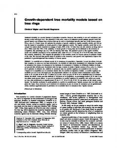
and forest turnover remains undefined. This gap in our knowledge stems mainly from the fact that earthquakes are unpredictable and stochastic phenomena [1,9], a problem that is exacerbated by limited field measurements. Earthquake–forest impact assessment has been improved dramatically from traditional field-based measurements to the use of advanced remote sensing techniques. Field investigation was the main method of data collection before remote sensing imagery became available [1,10]. However, because earthquakes often occur in mountainous areas and destroy roads, access to field sites is limited and the assessment of earthquake forest damage becomes difficult. The availability of satellite and aerial imagery has made it possible to estimate earthquake forest loss using remote sensing. The accuracy of remote sensing techniques depends on the affected area (i.e., gap size), and the spatial resolution of the remote sensors. Large gaps of disturbed forests are easily detected, while smaller areas can be found on remote sensing images with high spatial resolution [11]. The development of remote sensing analysis techniques, such as sub-pixel SMA (Spectral Mixture Analysis) [12], has made it possible to detect damaged areas that are smaller than one pixel in size. In addition, SMA utilizes all the spectral bands, which makes it more preferable than traditional green vegetation index, such as NDVI, which uses only two spectral bands and has relatively limited accuracy. SMA has been successfully applied to quantify tree mortality induced by hurricanes in recent years [4,13], and has great potential for detecting earthquake-induced forest loss. The 2008 Wenchuan earthquake was one of the strongest and most devastating seismic events in the last 50 years in China [14], resulting in substantial damage to the local environment and infrastructure. With a moment magnitude of 7.9, the Wenchuan earthquake occurred in a largely forested region, providing an opportunity to study the link between earthquakes, forest ecosystems and regional carbon dynamics. There are a few studies that have documented the impacts of Wenchuan earthquake on ecosystems [15–17]. However, the magnitude of such impacts is still a matter of controversy [18]. Large uncertainties exist in many earthquake-related forest loss estimates, mainly due to the use of imprecise impact boundary, methodological challenges and a lack of field inventory data. Qualitatively defining an impact boundary (e.g., political jurisdiction boundary) tends to bias estimation of earthquake-ecosystem effects. An earthquake impact estimation that objectively defines the affected area and appropriately integrates field data will therefore present the most accurate information about the impact of earthquakes on forest ecosystems. Here we integrated field measurements, satellite image analysis, seismic intensity fields and empirical mortality models to estimate the immediate impact of the Wenchuan earthquake on the forest ecosystems. The estimation of biomass loss is significantly improved by explicitly quantifying the earthquake impact boundary and using mortality models validated with detailed field measurements. Using a Monte Carlo simulation approach based on geographical information systems (GIS), we also calculated the earthquake-induced forest biomass carbon loss and its uncertainty. Our aim was to understand the regional effects and consequences of the earthquake and to provide reliable estimates for decision-making in forest management planning. 2. Materials and Methods 2.1. Study Area The Wenchuan earthquake occurred on 12 May 2008, with an epicenter (31.0˝ N, 103.4˝ E) located at the southern end of the Longmenshan Thrust Fault in southwestern China (Figure 1). It ruptured over 250 km of the fault and displaced the earth’s surface up to 3 m in many places [19]. Ground shaking caused mountain collapse and landslides, which induced even more damage to the local ecosystems. With the elevation ranging from 500 to 6000 m through the impact zone, there is a clear vertical distribution of forest beginning with subtropical forests at the base and subalpine conifer forests at the top of the mountains [20]. This heavily forested area plays an important role as a carbon sink in China [21].
Remote Sens. 2016, 8, 252
3 of 17
Remote Sens. 2016, 8, 252
3 of 17
Figure1.1.The The location location of earthquake andand fieldfield sample plots.plots. Figure ofWenchuan Wenchuan earthquake sample
2.2. Satellite Data Analysis
2.2. Satellite Data Analysis
Although the monitoring derived from high-resolution satellite images, such as Landsat TM or Althoughcould the monitoring derived fromofhigh-resolution satellite images, as Landsat TM or Quickbird, be more accurate, low levels spatial coverage and high costs limitsuch their applications. Quickbird, could be moreinaccurate, low levels of spatialarea coverage and high costs limit their applications. Moreover, the weather the Wenchuan earthquake-hit is most cloudy, and it is almost impossible to acquire images with less than area 20% is cloud temporal Moreover, thehigh-resolution weather in thesatellite Wenchuan earthquake-hit mostcoverage. cloudy, With and ithigher is almost impossible frequency, MODIS could provide images with much less cloud noise. Thus, larger coverage imagery of to acquire high-resolution satellite images with less than 20% cloud coverage. With higher temporal MODIS was used in the final estimation of forest mortality, and Landsat TM was utilized as a bridge to frequency, MODIS could provide images with much less cloud noise. Thus, larger coverage imagery of connect the MODIS-based mortality and field measured biomass loss. Landsat TM imagery (with MODIS was used in the final estimation of forest mortality, and Landsat TM was utilized as a bridge spatial resolution of 30 m) from 18 September 2007 and 18 July 2008 was used to estimate forest to connect the MODIS-based mortality and field measured biomass loss. Landsat TM imagery (with mortality for a small typical earthquake impact area. The Landsat derived mortality map was used to spatial resolution of of 30field m) from 18plots. September 2007 and July covered 2008 was estimate forest guide the location sample The mortality map,18 which theused entiretoearthquake mortality forareas, a small earthquake impact area.MODIS The Landsat derived map was used impacted wastypical generated from MODIS imagery. Terra images withmortality a spatial resolution to guide the location of field sample plots. The mortality map, which covered the entire of 250 m were selected from two dates, 9 May 2007 and 24 May 2008, to represent the pre- and earthquake postimpacted areas, was generated from MODIS imagery. MODIS Terra images with a spatial resolution earthquake conditions, respectively. Most of the Wenchuan areas are terrain. With the burial of and of 250 m were selected fromearthquake-influenced two dates, 9 May 2007 andmountainous 24 May 2008, to represent the predisturbed trees,conditions, the newly created bare lands increased the fragmentation of the land use. Thus, most post-earthquake respectively. pixels and MODIS imagery are combination different land cover. Here, With the spectral MostinofLandsat the Wenchuan earthquake-influenced areasofare mountainous terrain. the burial of mixture analysis was applied to extract different land cover. The reflectance of each pixel is assumed disturbed trees, the newly created bare lands increased the fragmentation of the land use. Thus, most to be the linear sum of the reflectance of different cover types weighted by their areal fractional pixels in Landsat and MODIS imagery are combination of different land cover. Here, the spectral presence within each pixel (Equations (1) and (2)).
mixture analysis was applied to extract different land cover. The reflectance of each pixel is assumed to m be the linear sum of the reflectance of different cover types weighted by their areal fractional presence ρib × Ci = ρb + ε b (1) within each pixel (Equations (1) and (2)).i =1
m ÿ i “1
ρmib ˆ Ci “ ρb ` ε b
C
i
= 1 .0
(2)
(1)
i =1
m ÿ
of pure end member i in wavelength where m is the number of end members, ρib is the C reflectance “ 1.0 i
band b (i.e., the reflectance of a pixel fully covered i“1 by end member i), Ci is the areal fraction of end member i in the focal pixel, ρb is the reflectance of the entire pixel in band b, Ɛb is the error of fit in
(2)
where m is the number of end members, ρib is the reflectance of pure end member i in wavelength band b (band residual). band b (i.e., the reflectance of a pixel fully covered by end member i), Ci is the areal fraction of end This work only focuses on forest ecosystem and its related biomass loss by the earthquake. A member i in the focal pixel, ρb is the reflectance of the entire pixel in band b, ε b is the error of fit in band forest pixel can usually be deconvolved into 4 basic cover types or end members (Figure 2): green b (band residual). vegetation (GV), non-photosynthetic vegetation (NPV, i.e., dead wood), soil, and shade [22]. The This workofonly on forest and its related biomassusing loss bya the earthquake. A forest reflectance thefocuses endmembers forecosystem Landsat imagery was extracted technique named pixel can usually be deconvolved into 4Cone basic(SMACC) cover types orwhereas end members (Figure 2): green Sequential Maximum Angle Convex [23], pixel purity index (PPI) vegetation was (GV), non-photosynthetic vegetation i.e., dead applied for the endmember extraction(NPV, from MODIS [24].wood), soil, and shade [22]. The reflectance of the endmembers for Landsat imagery was extracted using a technique named Sequential Maximum Angle Convex Cone (SMACC) [23], whereas pixel purity index (PPI) was applied for the endmember extraction from MODIS [24].
Remote Sens. 2016, 8, 252 Remote Sens. 2016, 8, 252
4 of 17 4 of 17 GV NPV
0.6
Soil
4 of 17
Shade
0.8
GV
0.4
Scaled Reflectance
Remote Sens. 2016, 8, 252
Scaled Reflectance
0.8
NPV
0.6
Soil
0.2
Shade
0.4
0.0 0.5
1.0
0.2
1.5
2.0
Wavelength (um)
0.0
Figure 2. The typical spectral 0.5 reflectance of Mixture Analysis. Analysis. used in Spectral Mixture 1.0the four endmembers 1.5 2.0 Wavelength (um)
Although NPV can represent dead wood, difference of NPV (or(or NPV + soil) of Although NPV can directly directly representofthe the dead wood,the the difference NPV NPV + soil) Figure 2. The typical spectral reflectance the four endmembers used in Spectral of Mixture Analysis. preand post-earthquake in fact had much less correlation with the field measured biomass loss of pre- and post-earthquake in fact had much less correlation with the field measured biomass loss based on on Although preliminary analysis. This might because because that thethe damaged trees were usually buried and NPVanalysis. can directly represent the deadthat wood, difference of NPV (orusually NPV + soil) of and based preliminary This might the damaged trees were buried demonstrated little NPV signal but more bare land signal. Therefore, instead of using NPV as a proxy pre- and post-earthquake in but fact more had much less correlation with the instead field measured demonstrated little NPV signal bare land signal. Therefore, of usingbiomass NPV asloss a proxy for dead wood as has been done in other studies [4,13], here we used the difference in green based on preliminary analysis. This might because that the damaged trees were usually buried and for dead wood as has been done in other studies [4,13], here we used the difference in green vegetation demonstrated little after NPV signal but more bare land signal.as Therefore, instead of using NPV asina each proxypixel. vegetation and the earthquake event measure of total losspixel. before and before after the earthquake event (∆GV) as a(ΔGV) measureaof total wood losswood in each Prior to for dead wood ΔGV, as hasthe been done in from otherall studies [4,13],were here shade-normalized we used the difference in green Prior to calculating GV values the images to limit effects calculating ∆GV, the GV values from all the images were shade-normalized to limit the the effects of vegetation before and after the earthquake event (ΔGV) as a measure of total wood loss in each pixel. of topography [22]. topography [22]. Prior to calculating ΔGV, the GV values from all the images were shade-normalized to limit the effects of topography [22]. 2.3. Extraction of Deciduous and Evergreen Forests
2.3. Extraction of Deciduous and Evergreen Forests
2.3. Extraction of Deciduous andpreliminary Evergreen Forests Coarse forested areas were were preliminary extractedbased basedon onthe theland landuse/land use/land cover cover map map of of China Coarse forested areas extracted China with a scale of 1/100,000 [25]. The land use map has six classes: agricultural fields, forests, grassland, with a scale of 1/100,000 [25].were Thepreliminary land use map has six classes: fields, grassland, Coarse forested areas extracted based on theagricultural land use/land coverforests, map of China waterwith areas, urban areas, fields. part appeared spectrally similar to a scale of 1/100,000 [25].open The land useSince map has sixofclasses: agricultural fields, forests, grassland, water areas, urban areas, and and open fields. Since part ofthe thegrassland grassland appeared spectrally similar forested pixels when validating on satellite images, both forests and grassland were extracted as water areas, urban areas, and open fields. Since part of the grassland appeared spectrally similar to to forested pixels when validating on satellite images, both forests and grassland were extracted as forested pixels when potentially forested areas.validating on satellite images, both forests and grassland were extracted as potentially forested areas. potentially forested areas. The potential potential forest forest areas were were further further classified classified as as deciduous deciduous and and evergreen evergreen based based on on their their The areas The potential forest areas were further classified as deciduous and evergreen based onvalue their after phenological difference, i.e., pixels with a high greenness value in the summer and a low phenological difference, i.e., pixels with a high greenness value in the summer and a low value after phenological difference, i.e., pixels with a high greenness value in the summer and a low value after senescence in the the winter winter were were classified classified as as deciduous, deciduous, while while pixels pixels that that maintained maintained aa certain certain level level of of senescence in senescence in the winter were classified as deciduous, while pixels that maintained a certain level of greenness throughout throughout the the year year were were classified classified as evergreen. evergreen. MODIS MODIS images images from from January January and and July July greenness greenness throughout the year were classified as as evergreen. MODIS images from January and July 2006 were used to represent the forest conditions in winter and summer, respectively. 2006 2006 were were used to represent the forest in winter summer, respectively. Both winter used to represent the conditions forest conditions in and winter and summer, respectively. Bothsummer winter and summer were bythe SMA, andthe the extracted GV values were used in and images wereimages processed byprocessed SMA, and extracted GV values used in forest Both winter and summer images were processed by SMA, and extracted GVwere values were used in type forest type classification, i.e., GV from winter image represents GV min while the GV from summer forest type classification, i.e., GV from winter image represents GV min while the GV from summer classification, i.e., GV from winter image represents GVmin while the GV from summer represents represents GVmax 3a). represents GV max (Figure 3a). GV (Figure 3a).(Figure max
(a)
A (a) (a)
(b)B
(b)
(b)B A ofof (a) Figure 3 The scatterplots plots of fraction green vegetation (GV) (GV) in summer and winter and the(a) forest Figure 3. The scatter fraction green vegetation in(b)summer and(a)winter and
the utility function (b). Points C and D represent ideal evergreen and deciduous forests, respectively; line forest utility function (b). Points C and D represent ideal evergreen and deciduous forests, respectively; Figure 3 The scatter plots of fraction of green vegetation (GV) in summer and winter (a) and the forest CD represents the ideal forest line.line. AC and represent relative probabilities for a pixel to contain line CD represents the ideal forest ACAD and AD represent relative probabilities for a pixelline to utility function (b). Points C and D represent ideal evergreen and deciduous forests, respectively; evergreen or deciduous forest. A pixel is assumed to be evergreen forest with a probability of AD/(AC contain evergreen deciduous forest. pixel assumed to be evergreen forest for with a probability of CD represents theor ideal forest line. ACAand ADis represent relative probabilities a pixel to contain + AD), and deciduous with a probability of AC/(AC + AD). AD/(AC AD), and deciduous ofbe AC/(AC + AD). evergreen+or deciduous forest. Awith pixelaisprobability assumed to evergreen forest with a probability of AD/(AC
+ AD), and deciduous with a probability of AC/(AC + AD).
Remote Sens. 2016, 8, 252
5 of 17
The ideal points for deciduous and evergreen were set based on the vegetation map, Google images, and field investigation (Figure 3a). The pure deciduous and conifer forests were delineated preliminarily based on the vegetation map and Google images. The areas were further refined by field investigation. The distributions of the GVmin and GVmax were constructed for the selected pure deciduous and conifer pixels, and the 95th percentile values of the GVmin and GVmax were taken as the ideal points. The GVmin and GVmax for the ideal point of deciduous were set to 0.002 and 0.83, respectively, while the two values for conifer were 0.69 and 0.75. The line connecting the ideal points of deciduous (D) and evergreen (C) represented ideal forest line (Figure 3a, Equation (3)) ax ` by ` c “ 0
(3)
where x and y are axis of GVmax and GVmin in Figure 3a, respectively. The parameters a, b and c are parameters calculated by ideal points of C and D in Figure 3a (Equations (4)–(6)). a “ GVmin‚C ´ GVmin‚D
(4)
b “ GVmax‚D ´ GVmax‚C
(5)
c “ pGVmax‚D ´ GVmax‚C q ˆ GVmin‚C ` pGVmin‚C ´ GVmin‚D q ˆ GVmax‚C
(6)
The likelihood that a pixel would be classified as forest was estimated by comparing its GVmin and GVmax to the forest ideal line. The points located to the right of the ideal forest line were assumed to be pure forests, whereas the points to the left were given probabilities based on their distances to the ideal line (Figure 3b, Equation (7)). Dist AB “
|a ˆ GVmax‚ A ` b ˆ GVmin‚ A ` c| ? a2 ` b2
(7)
The shorter the distance was, the higher probability the pixel would be classified as forest. The origin, with both GVmax and GVmin values of 0, was set as the least likelihood of 0 (Figure 3b). After a pixel was defined to be forest, another probability was calculated to categorize it as either deciduous or evergreen by a utility function based on its distances to the two ideal points. The distances of the pixel (A) to the ideal points (C and D) were calculated (i.e., AC and AD in Figure 3a). The comparison between the distances AC and AD determined the probability of forest type classification of pixel A. The pixel was assumed to be evergreen forest with a probability of AD/(AC + AD), and deciduous with a probability of AC/(AC+AD). The shorter the distance was, the higher the probability the pixel would be classified as the related forest type. 2.4. Quantifying the Total Impacted Area The earthquake impact boundary was estimated by comparing the ∆GV map with surface ground shaking experienced by the Wenchuan Earthquake (seismic intensity field). The seismic intensity of an earthquake is proportional to the degree of forest disturbance it causes, i.e., tree mortality declines with seismic intensity decreases. We calculated the distances of all the MODIS pixels to the Chinese seismic intensity isoline 10. The pixels located within isoline 10 (with seismic intensity > 10) were given negative distance values. The pixels were further grouped into bins based on their distances, and an average ∆GV value was calculated for each bin. It was assumed that ∆GV declined with the distance to isoline 10 until a turning point, after which ∆GV maintained a certain level regardless of the distance to isoline 10. The distance of the turning point could be the average maximum impact distance of the Wenchuan earthquake. 2.5. Ground-Based Tree Mortality Estimations The ∆GV map generated by the Landsat imagery was used to guide the locations of the field sample plots and to ensure them being randomly established across the entire disturbance gradient.
Remote Sens. 2016, 8, 252
6 of 17
The full range of ∆GV was classified into five levels (|t|)
Df
Sum of Square
Mean of Square
F Value
Pr (>F)
(a)
Deciduous
TM_∆GV (900 m2 )
12,737.9
604.1
21.09