Assessing preferential flow by simultaneously ... - Wiley Online Library

WATER RESOURCES RESEARCH, VOL. 49, 29–42, doi:10.1029/2012WR012148, 2013

Assessing preferential flow by simultaneously injecting nanoparticle and chemical tracers S. K. Subramanian,1 Yan Li,2 and L. M. Cathles1 Received 19 March 2012; revised 7 November 2012; accepted 8 November 2012; published 10 January 2013.

[1] The exact manner in which preferential (e.g., much faster than average) flow occurs in the subsurface through small fractures or permeable connected pathways of other kinds is important to many processes but is difficult to determine, because most chemical tracers diffuse quickly enough from small flow channels that they appear to move more uniformly through the rock than they actually do. We show how preferential flow can be assessed by injecting 2 to 5 nm carbon particles (C-Dots) and an inert KBr chemical tracer at different flow rates into a permeable core channel that is surrounded by a less permeable matrix in laboratory apparatus of three different designs. When the KBr tracer has a long enough transit through the system to diffuse into the matrix, but the C-Dot tracer does not, the C-Dot tracer arrives first and the KBr tracer later, and the separation measures the degree of preferential flow. Tracer sequestration in the matrix can be estimated with a Peclet number, and this is useful for experiment design. A model is used to determine the best fitting core and matrix dispersion parameters and refine estimates of the core and matrix porosities. Almost the same parameter values explain all experiments. The methods demonstrated in the laboratory can be applied to field tests. If nanoparticles can be designed that do not stick while flowing through the subsurface, the methods presented here could be used to determine the degree of fracture control in natural environments, and this capability would have very wide ranging value and applicability. Citation: Subramanian S. K., Y. Li, and L. M. Cathles (2013), Assessing preferential flow by simultaneously injecting nanoparticle and chemical tracers, Water Resour. Res., 49, doi:10.1029/2012WR012148.

1.

meter and submeter scale, are still not well understood in large part, because preferential flow is difficult to define and measure. Chemical tracers can diffuse into the stagnant zones fast enough that they appear to move through the subsurface more uniformly than they actually are. Deploying nanoparticles with a chemical tracer allows us to correct for this effect, and see more clearly the nonuniform nature of the flow. [3] The idea that tracers diffuse from flow fractures into adjacent matrix areas where flow is stagnant and that this can be inferred from the temporal changes in the concentration of produced tracers is by no means new. Becker and Shapiro [2000] summarize the extensive literature of modeling and field studies directed at explaining breakthrough tailing by tracer diffusion into matrix areas. They summarize some clear successes but also note that there are cases where tailing cannot be explained by diffusion and note that colloid tracer experiments have been disappointing to date because of low recovery. [4] The main problem with using particle tracers is the tendency of the particles to stick or otherwise be retained. Larger particles settle, are strained or filtered out in pore throats [McDowell-Boyer et al., 1986; Yao et al., 1971], or are caught in flow eddies. Numerous laboratory studies have investigated the mobility and retention of colloidal size particles in homogeneous soils, sands, and glass bead packed columns as a function of water chemistry, impurities, and contamination. Recent reviews [McCarthy and McKay, 2004; Ryan and Elimelech, 1996; Wan and Wilson,

Introduction

[2] Diverse fields such as groundwater contaminant migration, enhanced oil recovery, geothermal engineering, soil science, and radioactive waste management all need to understand flow through physical heterogeneities of different scales in the subsurface, and particularly how heterogeneities lead to preferential flow. Preferential flow can cause a toxic material to arrive at a sensitive location such as a drinking water aquifer much faster than expected, particularly if the toxic material is attached to a particle. Preferential flow can greatly reduce the effectiveness of a water flood by reducing the fraction of the oil-bearing rock that is swept. Fingering of cold recharge water into a geothermal system can degrade power output. Despite decades of effort, the causes of preferential flow, particularly on the

All Supporting Information may be found in the online version of this article. 1 Earth and Atmospheric Sciences, Cornell University, Ithaca, New York, USA. 2 KAUST-CU Center for Energy and Sustainability, Cornell University, Ithaca, New York, USA. Corresponding author: L. M. Cathles, Earth and Atmospheric Sciences, 2146, Snee Hall, Cornell University, Ithaca, NY 14853, USA. (lmc19@ cornell.edu) ©2012. American Geophysical Union. All Rights Reserved. 0043-1397/13/2012WR012148

29

SUBRAMANIAN ET AL.: NANOPARTICLE TRACERS

cal tracers together can measure the differential segregation of chemicals into a lower permeability matrix and reveal the degree of preferential flow. Experiments are carried out in four different laboratory apparatuses of three different designs. The experiments are interpreted by constructing sequestration plots that quantify the degree to which the tracers are retained in the apparatus, as tracer is passed through it. An inverse Peclet number is shown to predict when differential diffusional sequestration of the particle and chemical tracer can be expected. The sequestration plots indicate that there is significant flow through the matrix, and finite element models that include the slower flow into the matrix and the dilution it produces provide a more refined interpretation of the experiments. We show that the experimental data can be used to determine the core and matrix porosity, the longitudinal dispersion in the flow channels, and the transverse dispersion in the matrix, and that it is possible to interpret all the experiments with very similar parameter values. Particles measure dispersion parameters more effectively than chemical tracers. There is an indication that the C-Dots may be sticking to a slight degree, especially in the matrix, but the results clearly show that the diffusion of chemical tracer into the relatively stagnant matrix can be measured by simultaneously injecting chemical and particle tracers and noting the separation in the arrival times of the two in the effluent. Because preferential flow is such an important aspect of subsurface flow, the ability to measure it is important.

1994] summarize what is known about colloid aggregation, settling, straining, and deposition by filtration and the influence of physical and chemical heterogeneities. [5] Relatively, few studies have addressed particle transport in physically heterogeneous environments. The work that has been reported has mainly sought to explain the observation that radionuclides and toxic organic compounds can attach themselves to natural subsurface colloids and, as a result, be transported faster through fractures [Kanti Sen and Khilar, 2006; Kretzschmar et al., 1999; McCarthy and Zachara, 1989; Neretnieks, 1990; Ryan and Elimelech, 1996]. The papers we have found that are most relevant to our study are summarized in Table 1 and are discussed again at the end of this paper. Table 1 shows that only a small subset of published experiments have been carried out in a flow regime slow enough for diffusion to differentially affect the rate of transport of chemical and particle tracers. Only two laboratory experiments [Grisak et al., 1980; McCarthy et al., 2002] were run under conditions where enough time was allowed the chemical tracer to diffuse significantly into stagnant zones (e.g., an inverse Peclet number for the chemical tracer, NiPe, greater than one), and only one of these [McCarthy et al., 2002] deployed a particle as well as a chemical tracer and, thus, was able to demonstrate a separation in the effluent arrival times of the chemical and particle tracers. Four field experiments showed diffusional delays, but, in three of these cases, the particle tracers were strongly attenuated in their flow through the subsurface. Recently, Kanji et al. [2011] carried out a push–pull nanoparticle tracer field test in the Gawahar carbonate oil reservoir and recovered approximately 86% of injected tracer in approximately 7000 barrels of produced brine. Unfortunately, a chemical tracer was not simultaneously deployed in this experiment. [6] Nanoparticles such as metal oxides, carbon soot, and other organic complexes exist naturally in the subsurface. They can also be synthesized in a wide range of sizes and shapes [Wiesner and Bottero, 2007], from a wide range of materials (e.g., fullerene C-60, carbon, alumina, titania, and silica). More importantly, their surface can be decorated with host of different polymers and functional groups to provide stability in different solvents. Petosa et al. [2010] compile an exhaustive list of experimental studies carried out to understand and evaluate aggregation and deposition of different engineered nanomaterials in different porous media systems, and they also discuss the theoretical approaches currently being used to understanding the mechanisms behind the observed transport phenomena. [7] We have screened about a dozen nanoparticles for suitability as inert tracers and have found only a very few that do not stick or become otherwise retained in the simple glass bead packs used in our experiments. In the experiments reported here, we use a nanoparticle with a central spherical carbon core and a surface functionalized to make it water dispersible. These ‘‘C-Dots’’ are 2–5 nm in diameter and are thus much larger than molecules (0.1–1 nm) but smaller than all but the very smallest subsurface pores. The C-Dots are naturally photoluminescent with a high emission intensity that allows them to be detected at concentrations as low as approximately 0.01 ppm using a spectrofluorimeter. [8] This paper describes the design and interpretation of experiments that show how deploying particle and chemi-

2.

Experiments

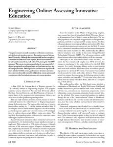
2.1. Experimental Design [9] Experiments were carried out in an apparatus of four different designs (three addressing preferential flow) as illustrated in Figure 1. Nanoparticles were first screened for their tendency to stick to the glass beads in a screening column (Figure 1a). The other designs all measure preferential flow, and the intent of each is to measure how diffusion from a core-flow channel into the stagnant matrix impacts the transmission of the tracers through the system. [10] In each preferential flow apparatus, there is a permeable core through which most of the flow occurs that is surrounded by a matrix within which the flow is much more stagnant. In some experiments, the ‘‘matrix’’ region adjacent to the core is compartmented by impermeable baffles that further discourage flow in the matrix. The cylindrical columns (Figures 1b and 1c) have a central channel of large diameter beads surrounded by an annulus filled with smaller diameter beads. The rectangular flow system (Figure 1d) has a lower channel filled with large beads which is covered with small beads. The Hele Shaw cell (Figure 1e) has a central rectangular core that is connected on one side by a fracture-like slit with much smaller aperture. [11] Water containing the tracer is injected directly into the core and collected from the core at the discharge end of the core in each system. The pore volume in the core is an important parameter in the analysis of system performance and will be referred to as the core pore volume. The total pore volume of the matrix will be referred to as the matrix pore volume. Table 2 lists these volumes for the flow systems in Figure 1. 30

0.0227

Niehren and Kinzelbach [1998] Becker et al. [1999]

31

0.0157

10.57

0.18

1.8

0.277

0.025

Bradford et al. [2004]

Cathles et al. [1974]

McKay et al. [2000]

McKay et al. [1993]

Neretnieks et al. [1982]

Grisak et al. [1980]

1.71

348

11.8

320

200

100

7.8

50

3

8.8

3.3

575

36

1000

0.091

50

1.74

1.41 0.0319

74.5

0.9

0.113

4.2

2

5

10

1

10

1.15

5

2.4

1

1

1

1.6

8

2.28

2.28

5.89

138.9

0.35

0.1

0.32

0.2

0.1

0.3

0.05

0.3

9.9

188

270

4.33

867

3.82

216

16.65

0.10 34.77

0.38

0.38

0.38

0.4

0.89

0.02

2.12

8.3

1.22

0.024

0.25

0.104

0.001

0.75

0.39

0.02

0.03

Delay

No separation

Separation

Separation

Separation

No separation

Separation

Separation

Separation

Separation

No separation

No separation

Small separation

Observation

Y

Y

Y

Y

Y

Y

Y

Y

N

Y

N

Y

Y

Agree

Lab, dual-porosity quartz sand packs Core, fractured tuff block Field, fractured granite Lab, dual-permeable quartz sand packs Field, fractured igneous rock Field, fractured saprolite Field, fractured clay till Core, cut fracture in granite core Core, fractured till

Core, fractured shale

Core, fractured shale

Core, cut fracture chalk Lab, quartz sand

‘‘Rock’’ Type

100 80

(CaCl2)

No particle tracers

No particle tracers

Very low recovery

Very low recovery

105 pulse (103) –

NaCl never recovered

Low recovery for large spheres Straining studied

Uranine delayed more than expected High recoveries

50 (0)

60 (100)

10.1 (80)

90 (80)

70 (94)

Pulse

0.14, 0.28, 1.4, 1 (100)

Core in cylindrical column Low concentrations indicate sticking and lack of clear separation Low recoveries

100 (100)

Comments Cut fracture

C/Co (%) 75, 100, 90 (92.5)

tritium oxide (THO)

Latex: 100, 500, 1000, 2100 nm (Br) Latex: 1000 nm (uranine) Latex: 280, 980 nm (I) Latex: 360, 830 nm (D2O) Latex: 1000, 3200 nm (Br) Silica spheres: 500 nm (Cl) Latex: 100 nm, bacteriophage (dye) Bacteriophage (Br)

Latex: 20, 200, 1000 nm (Br) Silica spheres: 100 nm (Cl) Latex: 50, 100, 500, 1000 nm (Br)

Tracer Particles (Chemical)

Parameters extracted from the papers and given in columns 2–6 are used to calculate a time-characterizing diffusion into the matrix, tdiff, and an inverse Peclet number (column 8) for the chemical tracer. As shown in later discussion in this paper, if NchemiPe approaches or exceeds one, a diffusionally delayed arrival of chemical tracer is expected, and a separation between the early arrival of the particle and the later arrival of the chemical tracer is expected. The ninth column records whether the observed separation is in agreement with the NchemiPe predictions. The analysis and implications of Table 1 are discussed in section 5. Symbols are defined: tc ¼ transit time through the preferential flow part of the system under the injection rate reported, Vt/Vc ¼ ratio of total to preferential flow pore volumes, ttotadv ¼ time for chemical tracer to transit the system if diffusion is very rapid and fills the matrix ¼ product of first two columns, H ¼ half the matrix width, m ¼ matrix porosity, tdiff ¼ time for chemical tracer to diffuse into matrix (equation (2)), C/Co ¼ maximum observed particle (and, in parentheses, chemical tracer) concentrations expressed as percentage of the tracer concentration injected.

a

1.07

Becker et al. [1999]

0.00579

0.23

McCarthy et al. [2002]

74.55

9.52

0.0118

0.012

203

0.0206

ttotadv tdiff NchemiPe ¼ tc (days) Vt/Vc (days) H (cm) m (days) ttotadv/tdiff

Cumbie and McKay [1999]

Zvikelsky and Weisbrod [2006] Saiers et al. [1994]

Reference

Table 1. Summary of Literature Describing Experiments Involving Chemical and/or Particle Tracers in Heterogeneous Porous Mediaa

SUBRAMANIAN ET AL.: NANOPARTICLE TRACERS

SUBRAMANIAN ET AL.: NANOPARTICLE TRACERS

Figure 1. Schematic of column designs. Dimensions are in centimeters. Schematics are not to scale. The (a) screening column, the (b and c) stainless steel and plexiglass cylindrical columns, the (d) rectangular beadpack system, and the (e) Hele Shaw flow system are shown. 2.3.2. KBr Tracer [14] The chemical tracer used in out experiments was reagent grade KBr (from ACROS, New Jersey, USA). The KBr diffusion constant is known from direct measurement and is about 2  105 cm2 s1 [Newman, 1973]. The effective diffusion constant is the aqueous diffusion constant multiplied by the bead pack porosity and divided by a tortuosity. For a bed of uniform spheres [Bear, 1972; Saffman and Taylor, 1958], a tortuosity of 1.5 is appropriate. The effluent concentrations were measured using an ion-selective electrode connected with a pH/mV/temperature microprocessor handheld meter (6230N, Jenco Instruments, California, USA). Prior to measuring the effluent concentration of KBr in each experiment, standard KBr solutions with known concentrations were prepared, and a calibration curve of KBr concentration as a function of electrode offset voltage was determined. The KBr concentration in the experiments was 1000 ppm. 2.3.3. Nanoparticle Tracer [15] The particles used in the experiments reported here, which we call Carbon Dots or C-Dots, are carbon-cored particles 2–5 nm in diameter, whose surface has been functionalized to be highly hydrophilic. As described by Krysmann et al. [2012], the particles are synthesized in a one-step thermal decomposition of citric acid monohydrate (Sigma Aldrich, St. Louis, USA) and ethanolamine (Sigma Aldrich) in a 1–3 molar ratio. The well-mixed solution is then heated under constant stirring to approximately 70 C until the water evaporates, and the residue is then pyrolyzed in air

2.2. Column Packing [12] All the systems were wet packed (e.g., the beads were introduced into a water-filled column) to ensure 100% water saturation. In the columns (Figures 1b and 1c), wire mesh was used to separate the coarse and fine glass beads. When baffles were used, thin, circular plexiglass sheets with the centers cut out were slid over the wire mesh core at regular intervals during the filling. The tubes were mechanically vibrated, as they were filled to ensure tight and uniform packing. In the rectangular bead packs (Figure 1d), no wire mesh separated the coarse and fine beads, and so, despite best efforts, there was inevitably some slight mixing of the beads at the interface, particularly for cases when this system was baffled by rectangular plexiglass sheets fitted into slits in the walls of the matrix portion of the cell.

2.3.

Materials

2.3.1. Glass Beads [13] The cylindrical columns and rectangular bead pack cells were packed with fine and coarse glass beads. The coarse beads were soda lime glass 3 or 1 mm in diameter, uniform in shape and size, and free of any visible stains or coloration. The fine beads were industrial quartz with an average diameter of 250 and 500 mm. These were washed repeatedly in deionized water until the pore water was clear and not turbid. The pore water pH was 6.8–7.0. Table 2. Dimensions of the Flow Systems Shown in Figure 1a Geometry

H (cm)

L (cm)

Core Pore Volume (cm3)

Matrix Slit Pore Volume (cm3)

Total Fluid Volume (cm3)

Homogeneous column (a) Hele Shaw cell (e) Rectangular bead pack: 10 compartments (d) Rectangular bead pack: 1 compartment (d) Plexicolumn (c) Stainless steel column (b)

NAb 4.8 7 7 1.4 0.92

54 20 15 15 50 50

NA 1.46 4.5 5.25 15.7 7.7

NA 7.78 36.8 31.5 195.2 81.9

14.8 9.24 41.3 36.75 210.9 89.6

a

H is the matrix width in cm and L is the length of the core in centimeters. The letter in parentheses in the first column refers to the diagram in Figure 1. Not applicable.

b

32

SUBRAMANIAN ET AL.: NANOPARTICLE TRACERS

C-Dots indicated by our experiments (as determined below) is approximately 1.5  106, which corresponds to approximately 3 nm based on Stokes-Einstein equation. [19] The ethanolamine polymer corona of the C-Dot particles is highly fluorescent. The concentration of the C-Dots is measured with a spectrofluorimeter (SpectraMax M2e, Molecular Devices, Sunnyvale, CA, USA). The excitation was at 370 nm, and the peak emission of the C-Dots is at 460 nm. Prior to measuring the effluent concentration of C-Dots in each experiment, standard C-Dots solutions were prepared, and a calibration curve of C-Dots concentration as a function of fluorescent intensity was determined. The effluent concentration of C-Dots was calculated using this calibration curve. 2.3.4. Other Particle Tracers [20] Commercial silica nanospheres of approximately 100 nm purchased from Corpuscular Inc. (Cold Spring, NY) were screened for possible use but rejected because they adhered to the glass beads. Rhodamine-6G dye was also considered as a tracer and rejected for two reasons. First, the large dye molecules have diffusion coefficients between 3.8  106 and 4.3  106 cm2 s1 [Muller et al., 2008], just slightly larger than our C-Dots. Second, as discussed below, the rhodamine stains the glass beads, and this adhesion substantially slows the transmission of the dye.

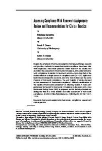
for various periods of time and at temperatures ranging from 200 C to 300 C, depending on the properties desired. The size of the C-Dots decreases until they agglomerate, as the duration and the temperature of the pyrolysis increase. The length of the ethanolamine polymer hairs attached to the carbon cores decreases with the pyrolysis temperature and duration. At low temperatures of pyrolysis, the fluorescence is very strong and associated with amide groups in the organic corona. At higher pyrolysis temperatures, the corona fluorescence decreases, and the fluorescence of the carbonic core increases and becomes dominant. The pyrolysis produces a black residue of functionalized nanoparticles that dissolves readily in water [Krysmann et al., 2012]. Our particles were pyrolyzed at 200 C for 8 h, dissolved in water, and used in the tracer tests reported without further purification. [16] The size of the particles dispersed in aqueous solution was determined with a Zetasizer Nano system (Malvern Instrument Ltd, Worcestershire, UK). The measurement is based on light scattering theory, and the size is inferred from the electrostatic mobility of the particles measured by laser. The zeta potential of the C-Dots is simultaneously determined. The C-Dot size determined in this fashion was 2–5 nm in diameter, and the zeta potential at pH 7 is 5 mV. [17] The C-Dots were examined in a transmission electron microscope (TEM) image as shown in Figure 2. The insert image shows that the size of the C-Dots is 2–5 nm. There is no significant particle aggregation, suggesting that the particles were well dispersed in solution. [18] The aqueous diffusion constant for the C-Dots can be calculated using the Stokes-Einstein equation: D1 ¼

kB T ; 3dp

2.4. Experimental Operation [21] The packed systems were flushed with 5–10 pore volumes of deionized water to ensure that the medium is completely saturated with water. A syringe pump connected to a three-way valve pushed water containing the tracers through the system. Effluent samples were collected over regular time intervals by an automatic sampler. The sampling interval was determined by the duration of the experiment, the expected transit time through the core channel, and the sample volume required for analysis. Upon completion of the experiment, deionized water was injected through the column for at least five to six total pore volumes or until the effluent concentrations reached the baseline levels for the tracers. If the concentration did not drop to baseline levels even after sustained injection of deionized water, or if a new particle tracer was being tested, the column was repacked. For the continuous injection experiments, around one total pore volume of tracer solution was usually injected through the column at a constant flow rate with a syringe pump. For the pulse injection experiments, a known quantity of tracer solution (generally about one fourth of a core pore volume) was injected into the system as a pulse and followed by injection of DI (distilled) water at the same flow rate.

(1)

where D1 is the aqueous diffusion coefficient in cm2 s1, kB is the Boltzmann constant (1.38065  1023 J K1), T is the absolute temperature (293.15 K), and dp is the diameter of the nanoparticle in cm, and  is the dynamic viscosity in g cm1 s1. Based on this equation, nanoparticles in the 2 to 5 nm diameter range indicated by the TEM images should have diffusion coefficients in the range of 2.1  106 and 8.6  107 cm2 s1. The diffusion constant for

3.

Figure 2.

Results

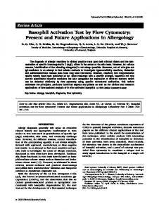
3.1. Screening for Stickiness with the Homogeneous Column [22] Figure 3a shows the results of screening the particles for their tendency to stick to the glass beads by passing four pore volumes of tracer through the homogeneous column illustrated in Figure 1a. The C-Dot and bromide tracer breakthrough (defined as the first detectable tracer in the effluent) occurs at approximately 1 pore volume, and the C-Dot concentration reaches 100% of injected concentration by approximately 1.1 pore volumes. The Rhodamine-6G breakthrough is delayed by nearly three fourth of

TEM image of C-Dots. 33

SUBRAMANIAN ET AL.: NANOPARTICLE TRACERS

Figure 3. C/Co versus number of pore volumes and time through a 500 mm glass bead homogeneous column (illustrated in Figure 1a). (a) Continuous injection of four pore volumes of tracer at a flow rate of 0.1 mL min1. (b) Injection of a 3 cm3 pulse of tracer followed by injection of four pore volumes of DI water at a flow rate of 0.1 mL min1.

a pore volume, however, and ultimately reaches only approximately 80% of the injected concentration. The 100 nm silica beads (S-100) tracer is also delayed but less so than the rhodamine tracer. Figure 3b shows that when a 3 cm3 (approximately one fifth of a pore volume) tracer pulse is injected at 0.1 cm3 min1, followed by DI water, the C-Dots and bromide tracers have almost identical breakthrough curves, but again the Rhodamine-6G and the S-100 tracers are delayed. The rhodamine tracer is clearly sticking to the glass beads. After injection, the beads can be seen to have a distinct red tint. We did not check for adhesion of the S-100 particles. Because of their adhesion, neither the S-100 nor rhodamine tracer is suitable for heterogeneous column experiments, and we do not consider them further in this paper. We mention them only to indicate how difficult it is to find a truly inert (nonsticky) tracer, even in systems as simple as glass bead packs.

3.2.2. Rectangular Bead Pack (Figure 1d) Experiments [25] Fluid was injected at one core pore volume per day. The system either had 1 (no baffles) or 10 (9 baffles) compartments. The 10 compartment case was run in continuous and pulse tracer injection modes. The single compartment experiment (Figure 4c) was run for 20 days and the multicompartment experiment (Figure 4d) for 6 days. In both cases, the C-Dots pass through the system faster than the bromide tracer and plateau at approximately 70%–80% of their injected concentration. In the one compartment case (Figure 4c), the bromide tracer curve crosses the C-Dot curve after about 1.5 total pore volumes of tracer has been injected. Figure 4e shows the C-Dots and bromide tracer concentrations when a pulse of 2 cm3 (approximately 2/5 core pore volume) is injected into the 10 compartment system, followed by approximately 7 days of water injection at one core pore volume per day. 3.2.3. Column Bead Pack (Figures 1b and 1c) Experiments [26] Figures 4f–4h show the results from the column experiments. As shown in Figure 4f, C-Dots arrive ahead of the KBr tracer when injected into the plexiglass (Figure 1c) column at approximately 1.8 core pore volumes per day but plateau at approximately 60%–70% of their injected concentration. By contrast, the bromide tracer reaches the injected concentration at about two total pore volumes of injection. When a 1/4 (2 cm3) core pore volume slug of KBr and C-Dot tracer is injected into the stainless steel column (Figure 1b) at 1.6 core pore volumes per day followed by DI water, C-Dot concentration peaks at 2% of the injected concentration and arrives at about two core pore volumes of injection, whereas the KBr tracer peaks at 1% of injected and arrives at about one total pore volume (Figure 4g). When a similar pulse is injected into the same column at 3.7 core pore volumes per day (Figure 4h), the results are similar but the KBr peak is lower. The material used to make the column is not important to the experimental results and is used here only for identification purposes.

3.2. Heterogeneous Column Experiments [23] Figure 4 plots the observed concentrations of bromide (blue circular data points) and C-Dot (red square data points) tracer in the effluent of all the experiments run as a function of the core pore volumes of fluid injected. A vertical line indicates when one total pore volume (core plus matrix pore volume) has been injected. Red and blue lines show the tracer concentrations predicted by the model used to interpret the data. Here, we describe the observed data. In the next section, we discuss their interpretation. 3.2.1. Hele Shaw Cell (Figure 1e) Experiments [24] The bromide and C-Dot tracers were injected at two very different flow rates. In both cases, the first breakthrough of tracer is at one core pore volume. When the tracers are injected at the low flow rate, the increase in bromide tracer in the effluent is significantly delayed compared to that of the C-Dot tracer (Figure 4a). By contrast, when the tracers are injected at a fast flow rate (Figure 4b), the concentration of the C-Dot and bromide tracers increase almost identically as a function of the number of core pore volumes of tracer injected, and the effluent tracer arrival curves overlap. 34

SUBRAMANIAN ET AL.: NANOPARTICLE TRACERS

Figure 4. Plot of observed effluent KBr (blue circles) and C-Dot (red squares) data points together with blue and red model curves (solid lines with compartment flow and dashed lines with no compartment flow). A vertical line indicates when one total pore volume has been injected. The parameters used in the compilation of the model curves are indicated in Table 4. Effluent tracer concentrations for the (a and b) Hele Shaw system, for the (c–e) rectangular beadpack flow system, for the (f) plexiglass column, and for the (g and h) stainless steel column are shown.

35

SUBRAMANIAN ET AL.: NANOPARTICLE TRACERS

4.

diffuse into the matrix during its transit through the core, and NiPe  1. If both the nanoparticle and chemical tracers have very small values of NiPe, they will have similar breakthrough curves. When the NiPe for KBr approaches and becomes larger than one, there is time for the tracer to significantly diffuse into the matrix during its transit through the flow system, and the tracer arrives close to one total pore volume, because it fills an appreciable fraction of the total porosity as it progresses through the tube. When the chemical tracer has NiPe  1 and the nanoparticle has NiPe  1, the tracer arrival curves are distinct, with the C-Dot tracer arriving at approximately 1 core pore volume and the KBr tracer arriving at approximately 1 total pore volume. [30] These relationships are clearly revealed by plots of the amount of tracer sequestered as a function of flow through the system. The fraction, f, of the total pore volume of the experimental system filled with tracer can be determined by integrating the product of the flow rate through the system (Q) and the difference between the tracer entering and exiting the system (1  C(t)/Co) over the duration of the experiment and dividing by the total pore volume of the system:

Interpretation

[27] The experimental results presented above are interpreted (1) first by comparing the tracer stored in the matrix to the amount of storage expected based on an inverse Peclet number and (2) then by comparing the observed effluent concentration curves to those predicted by a numerical model. 4.1. Interpretation With Sequestration Plots and an Inverse Peclet Number [28] The experiments described above show that tracers rise to concentrations similar to that injected at close to one core pore volume or one total pore volume, depending on the flow rate, diffusion coefficient, and geometry. This is because, for slower flow rates, there is more time for tracer to diffuse into the matrix where the flow is relatively stagnant (the Hele Shaw slit or the parts of the column and rectangular systems that are packed with small diameter beads), thereby delaying the tracer breakthrough. This can be analyzed using an inverse Peclet number, NiPe, defined by the ratio of the transit time of the fluid through the total porosity of the column to the time required for diffusion into the matrix: NiPe ¼

Z

Advection time constant  totadv ; ¼  diff Matrix diffusion time constant

  Dec Vt H2 ;  diff ¼ ; and Vc Dem Dem     aL c vc D1 c þ : ¼  m aT m vm

 totadv ¼ tc

f ¼

0

t

  CðtÞ dt Q 1 Co : Vtot

(3)

Here, C(t)/Co is the fraction of tracer measured in the effluent, and t is the time. If NiPe is very small, f should never significantly exceed the volume fraction represented by the core channel. If NiPe is around one, the fraction should approach the total pore volume of the system. [31] These relationships are schematically illustrated in Figure 5a. The lower dashed curve in Figure 5a indicates the sequestration that would be expected if there was no diffusion into the matrix at all. In this case, only the core channel needs to be filled with tracer before the tracer exits the system at the injected concentration, and there is no further tracer sequestration. The upper dashed curve indicates the sequestration that would be expected as tracer is injected if the diffusion of tracer into the matrix is extremely fast. In this case, the entire porosity of the system must be filled with tracer before the effluent tracer concentration reaches that injected and tracer sequestration ceases (the dashed line becomes flat). Cases where tracer diffusion into the matrix is neither zero nor very fast will lie between these two extremes, as illustrated by the red to blue solid curves. [32] Figures 5b–5d show the fraction of the total fluid volume that is filled with KBr (blue) or C-Dot (red) tracer as a function of the number of core pore volumes injected in the experiments shown in Figure 4. The plots are ordered so that NiPe (the ratio of to the full-porosity transit time to the matrix diffusion time constant) decreases from Figure 5b to 5d (from the top to the bottom of Figure 5). NiPe for each tracer is indicated on each plot. Each panel provides a reference to the effluent concentration plot in Figure 4. More information for each case is provided in Tables 3 and 4. [33] Several important features of the flow experiments are immediately apparent from Figure 5. First, except for the very fastest flow case at the bottom, the mass of

(2)

Here, the total advection time is the time for the tracer to move across the system assuming that the tracer fills the total porosity (the porosity of the channel and the matrix) as it progresses; tc is the transit time of fluid in the core channel (¼L/vc, where L is the length of the channel and vc is the average true velocity of fluid in the channel); Vt is the total pore volume of the whole system (core and matrix); Vc is the pore volume of the core channel, H is the width of the matrix; Dem and Dec are the effective diffusion coefficients in the matrix and core channel, respectively ;  is the tortuosity of the diffusion pathways around the beads (assumed to be the same in the matrix and channel); D1 is the aqueous diffusion constant of tracer; c and m are the porosities in the channel and matrix, respectively ; vm is the true velocity of the fluid in the matrix; and aL and aT are the longitudinal (parallel to flow) and transverse (perpendicular to flow) dispersion coefficients, respectively. Note that equation (2) assumes that only longitudinal dispersion is important in the channel and only transverse dispersion is important in the matrix. We write the equation this way because these are the assumptions we make in our numerical modeling as discussed in the next section. For the inverse Peclet number analysis, we neglect dispersion (e.g., assume aT ¼ aL ¼ 0); the sequestration plot analysis assumes there is no flow in the matrix. [29] At fast flow rates (low system residence times) or small diffusion constants, there is no time for a tracer to 36

SUBRAMANIAN ET AL.: NANOPARTICLE TRACERS

Figure 5. Storage and inverse Peclet number analysis of tracer bypass for C-Dots and KBr: (a) sequestration plot analysis and (b–f) tracer sequestered in the columns as a fraction of that which would fill the entire porosity (core channel and matrix). The NiPe values from Table 3 are shown for each curve. Annotations in each panel indicate the arrival time plot in Figure 4, which corresponds to the sequestration plot in Figure 5. is proportional to the permeability ratio of the core and matrix and is thus independent of the flow rate through the cell. The fraction of flow through the matrix (or Hele Shaw diffusion slit) is therefore not changed as the flow rate in the channel becomes large. The rise in the tracer curves above the lower dashed line channel box in Figure 5e shows this flow sequestration into the matrix directly. This flow must be addressed by our modeling, and we describe how this is done in the next section. [35] To our knowledge, plotting the tracer arrivals in the fashion illustrated in Figure 5 is new and is very useful. The plots clearly show that there is flow in the matrix in our laboratory experiments. If the fraction of tracer sequestered is greater than one, it is immediately apparent that the

bromide sequestered is more than the mass of C-Dots sequestered. Second, the fraction of tracer sequestered increases, as the NiPe increases (e.g., it is greatest for the slowest flow case at the top of Figure 5). Finally, there is some tracer sequestration in the matrix even if NiPe is very small (Figure 5d, bottom). [34] The last observation was unexpected and warrants some discussion. At very fast flow, the tracers should have no time to diffuse into the matrix and there should be no sequestration in the matrix. This will probably be the case in natural systems but is not the case in our laboratory system because the contrast in permeability between the channel and the matrix is not big enough that flow in the matrix is negligible. Furthermore, the flow rate through the matrix 37

SUBRAMANIAN ET AL.: NANOPARTICLE TRACERS Table 3. Operational Parameters for the Corresponding Experiments Highlighted in Figure 4a Geometry

Reference Figure

Nbr. Comp.

Tracers

Q (cm3 d1)

Duration (days)

Core Pore Volume Per Day (d1)

Hele Shaw cell (C) Hele Shaw cell (C) Rectangular bead pack (C) Rectangular bead pack (C) Rectangular bead pack (P-2cc) Plexicolumn (C) Stainless steel column (P-2cc) Stainless steel column (P-2cc)

4a 4b 4c 4d 4e 4f 4g 4h

13 13 1 10 10 11 1 1

C-Dot, KBr C-Dot, KBr C-Dot, KBr C-Dot, KBr C-Dot, KBr C-Dot, KBr C-Dot, KBr C-Dot, KBr

0.24 720 5.07 5.07 5.07 28.8 12 28.8

46 0.069 22.5 5.5 9 19 30 18

0.17 493 0.97 1.1 1.1 1.83 1.56 3.74

a Nbr. Comp., the number of compartments. (C) in the first column indicates continuous flow and (P) indicates pulse flow. Q is the flow rate through the column.

diffusional filling of the matrix would delay the arrival of a chemical compared to a particle tracer by 20%. The sequestration analysis must be made with a bit of insight and care.

porosities for the matrix or channel have been assigned incorrectly. The method should be immediately transferable to field interpretation of tracer experiments. In fractured rock, the total pore volume (fractures plus matrix porosity), matrix pore volume, and fracture spacing could be estimated from core data, and the inverse Peclet number could be estimated for particle and chemical tracers using the average flow rate in the fractures between wells, as was done by Cathles et al. [1974]. Where flow models are available, flow in stream tubes can be analyzed in this same fashion, and tracer arrivals predicted by summing the contributions of each stream tube connecting the injection and recovery wells. These methods, as well as a theoretical justification for the form of the inverse Peclet number we adapt here, will be published in a subsequent paper. [36] One final point on the sequestration analysis is as follows: if the fractures or flow zones are widely spaced, the diffusional relaxation time of the matrix will be long, and the NiPe could be small even though tracer might diffuse far enough into the matrix to affect its transit time. This is probably part of the explanation for the separation of the sequestration curves in Figures 5d and 5e despite the inverse Peclet numbers of both tracers being well less than one. The numerical model (discussed below) takes this issue, and also flows in the matrix, into account and matches the data fairly well. A way around the sequestration analysis dilemma of significant diffusion into wide matrix zones would be to pick a matrix thickness adjacent to the fractures that would slow the tracer arrival by a specified amount, say 20%, and define tdiff based on this thickness. When the NiPe for this matrix width is approximately one, partial

4.2. The Flow Model [37] The flow and transport of the tracers through the dual permeability core-slit and core-matrix systems can be modeled by calculating diffusion and flow separately using an operator splitting approach. In our model, the fluid is moved in small discrete steps (advancing one node per time step) along the core channel. At each step, tracer diffusion into the slit is calculated using finite element methods, and the concentration in the channel is appropriately reduced. Longitudinal dispersion and adsorption on the solid surface in the channel are included. Transverse dispersion is calculated in the matrix using the matrix fluid velocity profile calculated as described below. The longitudinal dispersion (DL) is calculated from the longitudinal (core-flow-parallel) true fluid velocity, vL : DL ¼ aLvL. The transverse (perpendicular to the flow velocity) dispersion in the matrix is calculated as follows: DT ¼ (aT/aL)aLvh, where aT/aL is the ratio of transverse to longitudinal dispersion, typically approximately 0.1. [38] The sequestration analysis shows that even when the slit is divided into sections by baffles, there is significant flow in the slit compartments. Flow from the channel enters the slit at the upstream end of each compartment and exits the slit at the downstream end of each compartment, as shown in Figure 6b. Until the entering fluid completes its circuit through the compartment, the entering fluid carries the tracer in, but the exiting fluid delivers no tracer out of, the compartment. This dilutes the tracer concentration

Table 4. Modeling Data and Best Fit Parametersa Geometry and Injection

Reference Figure

Nbr. Comp.

Q (cm3 d1)

c (%)

m (%)

aL (mm)

aT/aL

NiPe-C-Dot

NiPe-KBr

Hele Shaw cell (C) Hele Shaw cell (C) Rectangular bead pack (C) Rectangular bead pack (C) Rectangular bead pack (P) Plexicolumn (C) Stainless steel column (P) Stainless steel column (P)

4a 4b 4c 4d 4e 4f 4g 4h

13 13 1 10 10 11 1 1

0.24 720 5.07 5.07 5.07 28.8 12 28.8

100 100 35 30 30 40 40 40

30 30 30 35 35 37 35 35

0.1 0.1 4 4 4 4 4 4

0.1 0.1 0.1 0.1 0.1 0.25 0.25 0.25

0.21 7  105 0.004 0.004 0.004 0.11 0.23 0.09

2.81 9  104 0.06 0.06 0.06 1.42 3.10 1.29

a The tortuosity in the Hele Shaw experiments is one and for the bead packs 1.5. The aqueous diffusion constant for the KBr is 2  105 and for the C-Dots 1.5  106 cm2 s1. Abbreviations: (C) or (P) in the first column indicates continuous or pulsed flow; Q is the flow rate; aL is the longitudinal dispersivity; aT/aL is the ratio of transverse and longitudinal dispersivity; c and m are the porosity of core and matrix, respectively; and NiPe-C-Dot and NiPe-KBr are the inverse Peclet numbers computed from the parameters in Table 2 and the equations in the text for the C-Dot and KBr tracers, respectively.

38

SUBRAMANIAN ET AL.: NANOPARTICLE TRACERS

Figure 6.

Figure 7. The measured effluent C-Dot concentrations for the Hele Shaw (red squares) cell in the experiment shown in Figure 4a compared to model predictions for a range of C-Dot diffusion constants. The best fitting aqueous diffusion constant is 1.5  106 cm2 s1, and this value is within the range expected from the size of the particles (Figure 2) according to the Stokes-Einstein equation (equation (1)).

(a) Diffusion model and (b) cell flow model.

in water flowing through the channel. We compute this flow by calculating the permeability of the core and matrix using the Carmen-Kozeny equation for the bead packs or the Poiseuille flow equation for the Hele Shaw cell and by calculating the pressure drop along the channel from these permeabilities, apportion to flow in the core and matrix according to these permeabilities and the cross-sectional areas, and then use the methods of Toth [1962] and the linear pressure drop across the top of each compartment to calculate flow in the matrix (or Hele Shaw slit). For the Hele Shaw cell, the permeability of the square channel is the width squared divided by 32, and the permeability of the slit is its width squared divided by 12. We analytically determine the flow along a number of flow streamlines in the matrix (or slit) using the Toth equation, as illustrated in Figure 6, and calculate the time the flow takes to make the circuit along each streamline. The dilution is turned off for each streamline when the flow along that streamline completes its circuit through the compartment. Diffusion into the matrix is enhanced by adding dispersion to the matrix diffusion constant as indicted in equation (2). We take vm to be the horizontal fluid velocity in the matrix in the flowparallel middle of the compartment. This midline horizontal velocity decreases with distance from the channel into the matrix as determined by the Toth solution. [39] The model could account for tracer adhesion by requiring that a fraction of the tracer sticks to the solid surface before tracer is allowed to advance to the next computational node. We do not do this. We assume that there is no adhesion of the C-Dots or bromide ions to the solid surface as suggested by the homogeneous column tracer experiments. Taking account only of transverse dispersion in the matrix is an approximation that is warranted when the matrix compartments are wide compared to their depth, as they are in the single compartment cases, and flow in the matrix is almost entirely parallel to the core channel. The

model is approximate when the width to depth ratio of the compartments is less than one, and, in this case, advection and dispersion should be combined in the calculations, not treated separately by an operator splitting method as we have done. The model is approximate and could be improved, but it is nevertheless a substantial step toward a more sophisticated analysis of the experimental results, and it is adequate for our purposes in this paper. 4.2.1. Interpretation by Modeling Analysis [40] The aqueous diffusion constant of KBr is known and has a value of 2  105 cm2 s1, as reviewed above. This diffusion constant matches the KBr tracer data in the Hele Shaw cell experiments (as well as the other experiments). This provides some confirmation of our methods of analysis and justifies using the Hele Shaw data and the effluent curve for the C-Dot tracer to refine the aqueous diffusion constant for the C-Dots from the range of values their size and the Stokes-Einstein equation would predict. Figure 7 shows the best fitting aqueous diffusion constant of the C-Dots that is equal to 1.5  106 cm2 s1, and we use this value in the analysis of our experimental data. As reviewed above, the diffusion tortuosity of a spherical bead pack is known to be 1.5, and we use this value in both the channel and matrix for the experiments where the apparatus was filled with glass beads. For the Hele Shaw cell, tortuosity is assumed to be one. In other words, in our interpretation of the experimental data, we assume that D1-C-Dot ¼ 1:5  106 cm2 s1 , D1-KBr ¼ 2  105 cm2 s1 , and  ¼ 1.5 (bead packs) and  ¼ 1 (Hele Shaw). [41] The parameters that remain to be constrained by the experimental data are the porosity and the dispersion constants in the channel and matrix ðc ; m ; aL ; and aT Þ as indicated in Table 4. Parametric plots in the Supporting 39

SUBRAMANIAN ET AL.: NANOPARTICLE TRACERS

[45] Figures 4g and 4h show how models fit the pulse test data in a one compartment stainless steel column carried out at two different flow rates (12 and 28.8 mL d1). The column core (40%) porosity is the same as for the 11-compartment plexiglass column, but the matrix porosity is 35% compared to 37% for the plexiglass column. The model fits the data at the two different flow rates well for the same parameters. [46] The Supporting Information presents four summary tables and 56 plots documenting how the experiments constrain the porosity of the core and matrix, the longitudinal dispersivity in the channel, and the transverse dispersivity in the matrix. The best fitting matrix porosity (m) ranges from 30% to 37%. The best fitting core porosity (c) varies with experiment type and number of compartments between 30% and 40% and is less well constrained than the matrix porosity. The longitudinal dispersion parameter is 0.1 mm for the Hele Shaw experiments and 4 mm for all the experiments involving glass beads. The dispersion in the Hele Shaw case is constrained only by high flow rate CDot and KBr experiment, as expected from equation (2). The longitudinal dispersion in the bead experiments is constrained best by the C-Dots in the pulse experiments. The same is true for the aT/aL ratio.

Information are summarized in Table ES2. These plots document how the core and matrix porosities in Table 4 are determined by modeling the experimental data. The solid model curves in Figure 4 (blue for the KBr and red for the C-Dot tracers) demonstrate the quality of the match between the experimental data and the model predictions that can be achieved with the parameters recorded in Table 4. The dashed lines (labeled no compartment flow) in Figure 4 show the effluent concentration history if flow into the compartments is not included in the model. The difference between the dashed and solid lines shows the importance of taking flow in the matrix into account, as is done for the solid lines. [42] The model curves fit the Hele Shaw cell data (Figures 4a and 4b) very well at both fast and slow flow rates. The KBr line shows that the model fit is good using the literature value for the aqueous diffusion constant of KBr. The dashed lines, which do not take into account flow in the matrix, lie far from the data points and show the importance of taking into account the flow in the matrix. The best fit data for C-Dots (Figure 4a) are obtained for a diffusion coefficient of approximately 1.5  106 cm2 s1. This is demonstrated in the Supporting Information. [43] Figures 4c–4e show that the model also fits the experiments in the rectangular bead pack quite well for both continuous and pulse flows and for the same parameters that were successful in simulating the tracer transmission in the Hele Shaw cell (Table 4). Taking into account flow in the matrix is again important (difference between the dashed and solid model lines). The longitudinal dispersivity aL approximately 4 mm gives the best fit to the experimental data, but this parameter is best constrained by data on the 10 compartment bead pack. The best fitting porosity of the channel is greater for the one compartment case (Figure 4c, c ¼ 35%) than for the 10 compartment case (Figures 4d and 4e, c ¼ 30%). This could be due to the packing methods described in section 2. In multicompartment cells, there could be more entrainment of fine glass beads into the channel because each baffled compartment must be filled separately. Intermixing has been observed while packing the columns, and it is not unusual for visible intermixing to require repacking. The model KBr curve does not cross the C-Dot curve as observed. This suggests that there may be some sticking and retention of nanoparticles in the matrix that is not taken into account in the model. [44] Figures 4f shows that the model simulations match the plexiglass column data. The model fit for the KBr and C-Dot data is not perfect. The KBr model curve predicts a slightly earlier arrival history than the data show; the C-Dot model predicts a slightly later arrival history than the data show. The C-Dot model predicts higher concentrations than are observed in later times, suggesting there may be some sticking of C-Dot particles. The porosity of the core is greater than for bead pack experiments (c ¼ 40% rather than 30%–35%), and the porosity of the matrix is greater (h ¼ 37% rather than 30%–35%). The higher core porosity is reasonable because the cylindrical column cores are protected from mixing with the fine beads by a screen. The transverse dispersion for the cylindrical columns is greater than the rectangular bead pack (aT/aL ¼ 0.25 rather than 0.1). We think that this is probably due to less perfect packing in the matrix near the core channel.

5.

Summary and Discussion

[47] The experiments reported here were designed to test whether dual-tracer experiments can measure preferential flow from the differential transit of tracers across a system in which diffusion can occur into relatively stagnant areas adjacent to the areas of preferential flow. The results show preferential flow is clearly indicated by the more rapid transport of nanoparticles compared to chemical tracer. [48] The concentrations of C-Dots and KBr were estimated using a spectrofluorimeter and an ion selective electrode, respectively. The effluent concentration data are interpreted using a sequestration analysis and by numerical simulation of advection and dispersion. The sequestration plots in Figure 5 show that tracer sequestration into the matrix increases, as the inverse Peclet number, NiPe, increases. Because the plots show sequestration in the matrix at very low NiPe, when there should be very little diffusion into the matrix, they also clearly indicate that there is flow into the matrix in the laboratory experiments. [49] Modeling the experimental data with more sophisticated (but still approximate) operator splitting numerical methods that take into account flow in the matrix, we find that all the experimental data can be explained quite well by a common set of parameter values. It is clearly important to take into account flow in the matrix. With this flow accounted for, all the experimental data are fit with a narrow and reasonable range of parameters as summarized in Table 4 and the discussion at the end of the preceding section. Variations in column porosities and dispersion constants are reasonable and within the limits of the construction and filling with beads of the experimental apparatus. Slight parameter differences (such as the transverse dispersion in the matrix and slightly different matrix and core porosities) that are required to fit the column tracer data probably arise from the difficulty in uniformly packing these columns that 40

SUBRAMANIAN ET AL.: NANOPARTICLE TRACERS

a high reduction in concentration due to filtration, straining in pore throats, eddy sequestration, or other processes such as sticking. Moreover, as commented earlier, our experience is also showing that it is difficult to find nanoparticles that do not stick. The relatively small size of our successful 2–5 nm C-Dots means that they should not gravitationally settle. However, small particles tend to have almost no secondary attractive minima, and their repulsive barrier is also small [Petosa et al., 2010; Wiesner and Bottero, 2007]. On this basis, small particles are expected to stick more than large ones. Also, it is thought that small particles (with higher Brownian motion) tend to agglomerate with each other or stick to the solid surface more than larger particles. On the other hand, Kobayashi et al. [2005] have shown that, physical and chemical conditions being the same, smaller nanoparticles appear slightly more stable than the larger ones. Our experiments suggest that, for whatever reason, our small C-Dot particles stick remarkably little to the glass beads used in our experiments. We are currently investigating the reasons for this relatively high dispersibility and nonstickiness. [53] The tracer experiments discussed here show that dual (particle and inert chemical) tracers can measure fluid bypass in the laboratory. The fluid residence times in our experiments were much longer than in most previous laboratory-scale literature studies where the flow rates were typically at least 10–100 times faster than ours. Bypass is immediately apparent from sequestration plots and inverse Peclet number analysis, and these methods, as well as the finite element methods we discuss, can be transferred to the interpretation of field experiments. The laboratory data, together with two successful field experiments [Cathles et al., 1974; Kanji et al., 2011], strongly suggest that nanoparticles can be used to measure fluid bypass in the field. The small size of our C-Dot particles appears to allow them to avoid sticking and filtration and explain the high recoveries obtained in our experiments.

are exacerbated by the fact that the interface between the matrix and core is hidden during filling. [50] The best fit diffusion constant for C-Dots (1.5  106 cm2 s1) suggests a particle size approximately 3 nm, which is within the 2 to 5 nm size range indicated in the TEM images of C-Dots. The lower-than-modeled concentration of the C-Dots at the later times in the continuous injection glass bead experiments may indicate a slight sticking of the particles. The match in early times can be slightly improved by adding a small degree of sticking. The lower-than-predicted effluent concentration at the later times almost certainly indicates a slight particle loss during flow through the matrix, which our model does not account for. Overall, what is remarkable, however, is how well the data can be modeled with only minimal and reasonable variations of a common set of parameters. [51] The inverse Peclet number is applied to interpreting experiments reported in the literature in Table 1. We constructed this table by determining the following parameters for each experiment: (1) the fluid transit time (tc in column 2) through the preferential flow part of the system (the fracture, permeable central core, fracture porosity, etc.) and (2) the ratio of the total pore volume to the fracture(s) or permeable zone (Vt/Vc in column 3), half the matrix width (H in column 4), and the matrix porosity (m in column 5). We then calculated the transit time for the condition in which the tracer diffuses rapidly into the matrix (tc times Vt/Vc) and the diffusional time constant for the chemical tracer, tchemdiff, using equation (2). We then compute the inverse Peclet number for the chemical tracer, NchemiPe, from the ratio of these two parameters. If NchemiPe approaches or exceeds one for the chemical tracer, we expect to see a delay in the arrival of the chemical relative to the particle tracer. Column 10 indicates whether the experiment behaves according to this expectation. It can be seen that of the 13 experiments tabulated, only two contradicted our expectations regarding diffusion. For one of these [Niehren and Kinzelbach, 1998], there are clear indications that the uranine is sticking to the quartz sand. The pore volume in the impermeable filters is not sufficient to account for the observed delay in the uranine tracer. We have no good explanation for the failure of the latex spheres in the experiment by Cumbie and McKay [1999] to arrive earlier than the KBr tracer other than that there was very low recovery of the latex spheres, and the spheres may have been delayed by sticking to a mineral surface in the shale. The clearest diffusional delay is shown by McCarthy et al. [2002] who inject a tracer pulse through fractured shale, but the recovery of the particles was very low. Three of the four field tests are expected to, and do, show a clear delay in the arrival of the chemical tracer, but the recovery of the particles in three of these tests was very low, and the fourth was perhaps compromised by chemical alteration of the particles before they were all analyzed [Cathles et al., 1974]. Table 1 shows that although very few relevant experiments have been carried out, those that have been carried out are in good accord with the diffusional sequestration that is expected based on an easily calculated inverse Peclet number, NiPe. [52] The C-Dots in our experiments show very low retention compared to colloids transported through different porous media systems. This is remarkable in light of the literature experience showing colloid tracers usually suffer

5.1. Recommendations [54] For the future, it will be important to understand better the reasons that nanoparticles do not stick. Nanoparticles with the same surface charge but of different sizes (within 1 to 100 nm domain) should be tested for retention under constant geochemical conditions. Particle stickiness as a function of solution chemical parameters such pH, ionic strength, and the concentration of specific (especially divalent) counterions needs to be investigated. The zeta potential of a mineral is known to depend on solution chemistry. Glass beads are a poor proxy for carbonates, silicates, and clays. Stickiness should be investigated for the range of minerals commonly encountered in the subsurface. Special surface coatings that add a layer of molecular chains can significantly enhance the stability of the particles, and this steric enhancement is more significant for smaller particles (sub-10 nm) than particles which are larger. Studies have shown that these kinds of coatings can reduce sticking to surfaces [Wan and Wilson, 1994]. A more detailed study of the degree of particle sticking as a function of surface coating might help in better understand the stability and nonsticky nature of 1–10 nm sized particles. As highlighted by Petosa et al. [2010], there is a need to bridge the gap between the theories applied to 41

SUBRAMANIAN ET AL.: NANOPARTICLE TRACERS Kretzschmar, R., M. Borkovec, D. Grolimund, and M. Elimelech (1999), Mobile subsurface colloids and their role in contaminant transport, in Advances in Agronomy, edited by L. S. Donald, pp. 121–193, Academic, New York. Krysmann, M. J., A. Kelarakis, P. Dallas, and E. P. Giannelis (2012), Formation mechanisms of carbogenic nanoparticles with dual photoluminescence emission, J. Am. Chem. Soc., 134, 747–750. McCarthy, J. F., and L. D. McKay (2004), Colloid transport in the subsurface—Past, present, and future challenges, Vadose Zone J., 3(2), 326– 337. McCarthy, J. F., and J. M. Zachara (1989), Subsurface transport of contaminants, Environ. Sci. Technol., 23(5), 496–502. McCarthy, J. F., L. D. McKay, and D. D. Bruner (2002), Influence of ionic strength and cation charge on transport of colloidal particles in fractured shale saprolite, Environ. Sci. Technol., 36, 3735–3743. McDowell-Boyer, L. M., J. R. Hunt, and N. Sitar (1986), Particle transport through porous media, Water Resour. Res., 22, 1901–1921. McKay, L. D., R. W. Gillham, and J. A. Cherry (1993), Field experiments in a fractured clay till: 2. Solute and colloid transport, Water Resour. Res., 29(12), 3879–3890. McKay, L. D., W. E. Sanford, and J. M. Strong (2000), Field-scale migration of colloidal tracers in a fractured shale saprolite, Ground Water, 38(1), 139–147. Muller, C. B., A. Loman, V. Pacheco, F. Koberling, D. Willbold, W. Richtering, and J. Enderlein (2008), Precise measurement of diffusion by multi-color dual-focus fluorescence correlation spectroscopy, Europhys. Lett., 83(4), 46001. Neretnieks, I. (1990), Solute Transport in Fractured Rock: Applications to Radionuclide Waste Repositories, Svensk k€arnbr€anslehantering, Stockholm. Neretnieks, I., T. Eriksen, and P. T€ahtinen (1982), Tracer movement in a single fissure in granitic rock: Some experimental results and their interpretation, Water Resour. Res., 18(4), 849–858. Newman, J. (1973), Electrochemical Systems, 432 pp., Prentice-Hall, Englewood Cliffs, N. J. Niehren, S., and W. Kinzelbach (1998), Artificial colloid tracer tests: Development of a compact on-line microsphere counter and application to soil column experiments, J. Contam. Hydrol., 35(1–3), 249–259. Petosa, A. R., D. P. Jaisi, I. R. Quevedo, M. Elimelech, and N. Tufenkji (2010), Aggregation and deposition of engineered nanomaterials in aquatic environments: Role of physicochemical interactions, Environ. Sci. Technol., 44(17), 6532–6549. Ryan, J. N., and M. Elimelech (1996), Colloid mobilization and transport in groundwater, Colloids Surf. A: Physicochem. Eng. Aspects, 107(Compendex), p. 56. Saffman, P. G., and G. Taylor (1958), The penetration of a fluid into a porous medium or Hele-Shaw cell containing a more viscous liquid, Proc. R. Soc. A: Math., Phys. Eng. Sci., 245(1242), 312–329. Saiers, J. E., G. M. Hornberger, and C. Harvey (1994), Colloidal silica transport through structured, heterogeneous porous media, J. Hydrol., 163(3–4), 271–288. Toth, J. (1962), A theory of groundwater motion in small drainage basins in central Alberta, Canada, J. Geophys. Res., 67(11), 4375–4387. Wan, J., and J. L. Wilson (1994), Colloid transport in unsaturated porous media, Water Resour. Res., 30(4), 857–864. Wiesner, M. R., and J.-Y. Bottero (2007), Environmental Nanotechnology: Applications and Impacts of Nanomaterials, McGraw-Hill, New York. Yao, K.-M., M. T. Habibian, and C. R. O’Melia (1971), Water and waste water filtration. Concepts and applications, Environ. Sci. Technol., 5(11), 1105–1112. Zvikelsky, O., and N. Weisbrod (2006), Impact of particle size on colloid transport in discrete fractures, Water Resour. Res., 42(12), W12S08, doi:10.1029/2006WR004873.

colloids and molecules to better understand and evaluate the stability and transport of nanoparticles in the 1 to 10 nm size range. [55] We have a lot to learn about particle stickiness, but, in closing, it is worth emphasizing how significant it would be if we could develop nonsticking nanoparticles that could be used to identify preferential flow in fractured rock and sediments. This capability would find many applications in enhanced oil recovery, geothermal engineering, soil science, contaminant transport, and radionuclide waste management, and it could enable new strategies for subsurface flow engineering and remediation. The ultimate goal in the development of dual tracer capabilities for measuring fluid bypass must be to run dual tracer nanoparticle experiments in the field. The laboratory experiments we report here show the promise, but we need field-capable nanoparticle tracers. The relatively low retention of inert C-Dots (compared to other literature studies, our own screening tests, and as indicated by the Aramco field test) provides encouragement that particle-chemical tracers will be successful in the field and ultimately provide an entirely new tool for measuring and understanding heterogeneous subsurface flow. [56] Acknowledgments. This publication was based on work supported by award KUS-C1-018-02, made by King Abdullah University of Science and Technology (KAUST).

References Bear, J. (1972), Dynamics of Fluids in Porous Media, Elsevier, New York. Becker, M. W., and A. M. Shapiro (2000), Tracer transport in fractured crystalline rock: Evidence of nondiffusive breakthrough tailing, Water Resour. Res., 36(7), 1677–1686. Becker, M. W., P. W. Reimus, and P. Vilks (1999), Transport and attenuation of carboxylate-modified latex microspheres in fractured rock laboratory and field tracer tests, Ground Water, 37(3), 387–395. Bradford, S., M. Bettakhar, J. Simunek, and M. Genuchten (2004), Straining and attachment of colloids in physically heterogeneous porous media, Vadose Zone J., 3, 384–394. Cathles, L., H. Spedden, and E. Malouf (1974), A tracer technique to measure the diffusional accessibility of matrix block mineralization, Am. Inst. Mining, 103rd Annu. Meet., 1974, 19 pp. Cumbie, D. H., and L. D. McKay (1999), Influence of diameter on particle transport in a fractured shale saprolite, J. Contam. Hydrol., 37(1–2), 139–157. Grisak, G. E., J. F. Pickens, and J. A. Cherry (1980), Solute transport through fractured media: 2. Column study of fractured till, Water Resour. Res., 16(4), 731–739. Kanji, M., Y. K., H. Rashid, and E. Giannelis (2011), Industry first field trial of reservoir nanoagents, in SPE Middle East Oil and Gas Show and Conference, p. 10, Society of Petroleum Engineers, Manama, Bahrain. Kanti Sen, T., and K. C. Khilar (2006), Review on subsurface colloids and colloid-associated contaminant transport in saturated porous media, Adv. Colloid Interface Sci., 119(2–3), 71–96. Kobayashi, M., F. Juillerat, P. Galletto, P. Bowen, and M. Borkovec (2005), Aggregation and charging of colloidal silica particles: Effect of particle size, Langmuir, 21(13), 5761–5769.

42