Sep 7, 2017 - proven useful for text classification tasks (Tai et al.,. 2015; Tang et al., .... The BIDIRECTIONAL LSTM (BILSTM) has the same architecture as the ...
Assessing State-of-the-Art Sentiment Models on State-of-the-Art Sentiment Datasets Jeremy Barnes, Roman Klinger, and Sabine Schulte im Walde Institut f¨ur Maschinelle Sprachverarbeitung University of Stuttgart Pfaffenwaldring 5b, 70569 Stuttgart, Germany {barnesjy,klinger,schulte}@ims.uni-stuttgart.de
Abstract
Internet (Forsyth and Martell, 2007). The first approaches in this field of research depended on the use of words at a symbolic level (unigrams, bigrams, bag-of-words features), where generalizing to new words was difficult (Pang et al., 2002; Riloff and Wiebe, 2003). Current state-of-the-art methods rely on features extracted in an unsupervised manner, mainly through one of the existing pre-trained word embedding approaches (Collobert et al., 2011; Mikolov et al., 2013; Pennington et al., 2014). These approaches represent words as some function of their contexts, enabling machine learning algorithms to generalize over tokens that have similar representations, arguably giving them an advantage over previous symbolic approaches. In order to evaluate state-of-the-art models (both symbolic and embedding-based), different datasets are used. However, it is not clear that a model that performs well on one certain dataset will transfer well to other datasets with different properties. The work we describe in this paper aims at discovering if there are certain models that generally perform better or if there are certain models that are better adapted to certain kinds of datasets. Ultimately, the goal of this paper is to contribute to the current situation by supporting the choice of a method for novel domains and datasets, based on properties of the task at hand. Our main contributions are, therefore, comparing seven approaches to sentiment analysis on six benchmark datasets1 . We show that • bidirectional LSTMs perform well across datasets, • both LSTMs and bidirectional LSTMs are particularly good at fine-grained sentiment tasks, • and embeddings trained jointly for semantics
There has been a good amount of progress in sentiment analysis over the past 10 years, including the proposal of new methods and the creation of benchmark datasets. In some papers, however, there is a tendency to compare models only on one or two datasets, either because of time restraints or because the model is tailored to a specific task. Accordingly, it is hard to understand how well a certain model generalizes across different tasks and datasets. In this paper, we contribute to this situation by comparing several models on six different benchmarks, which belong to different domains and additionally have different levels of granularity (binary, 3-class, 4-class and 5-class). We show that BiLSTMs perform well across datasets and that both LSTMs and Bi-LSTMs are particularly good at fine-grained sentiment tasks (i. e., with more than two classes). Incorporating sentiment information into word embeddings during training gives good results for datasets that are lexically similar to the training data. With our experiments, we contribute to a better understanding of the performance of different model architectures on different data sets. Consequently, we detect novel state-of-the-art results on the SenTube datasets.
1
Introduction
The task of analyzing private states expressed by an author in text, such as sentiment, emotion or affect, can give us access to a wealth of hidden information to analyze product reviews (Liu et al., 2005), political views (Speriosu et al., 2011), or to identify potentially dangerous activity on the
1
The code and embeddings for the best models are available at http://www.ims.uni-stuttgart.de/ data/sota_sentiment
2
Proceedings of the 8th Workshop on Computational Approaches to Subjectivity, Sentiment and Social Media Analysis, pages 2–12 c Copenhagen, Denmark, September 7–11, 2017. 2017 Association for Computational Linguistics
and sentiment perform well on datasets that are similar to the training data.
2
in this paper as R ETROFIT). They require a vocabulary V = {w1 , . . . , wn }, its word embedˆ = {ˆ dings matrix Q q1 , . . . , qˆn }, where each qˆi is one vector for one word wi and an ontology Ω, which they represent as an undirected graph (V, E) with one vertex for each word type and edges (wi , wj ) ∈ E ⊆ V × V . They attempt to learn the matrix Q = {q1 , . . . , qn }, such that qi is similar to both qˆi and qj ∀j for (i, j) ∈ E. Therefore, the objective function to minimize is " # n X X 2 2 Ψ(Q) = αi ||qi −ˆ qi || + βi,j ||qi −qj || ,
Related Work
This section discusses three approaches to sentiment analysis and then describes in detail benchmark datasets which will be used in the experiments. 2.1
Approaches
To analyze the performance of state-of-the-art methods across datasets, we experiment with three approaches to sentiment analysis: (1) updating pretrained word embeddings using a neural classifier and labeled data, (2) updating pre-trained word embeddings using a semantic lexicon, and (3) training word embeddings to jointly maximize a language model score and a sentiment score. Sections 2.1.1 to 2.1.3 discuss these three approaches. We focus on sentiment-related methods, however, where appropriate, we discuss general approaches which can be adapted to this use case in a straightforward manner as well. 2.1.1
i=1
(i,j)∈E
where α and β control the relative strengths of associations. They use the XL version of the Paraphrase Database (PPDB-XL) dataset (Ganitkevitch et al., 2013), which is a dataset of paraphrases as the semantic lexicon, to improve the original vectors. This dataset includes 8 million lexical paraphrases collected from bilingual corpora, where words in language A are considered paraphrases if they are consistently translated to the same word in language B. They then test on the Stanford Sentiment Treebank (Socher et al., 2013). They train an L2regularized logistic regression classifier on the average of the word embeddings for a text and find improvements after retrofitting. All above approaches show improvements over previous word embedding approaches (Mnih and Teh, 2012; Yu and Dredze, 2014; Xu et al., 2014) on this data set.
Retrofitting to Semantic Lexicons
There have been several proposals to improve the quality of word embeddings using semantic lexicons. Yu and Dredze (2014) propose several methods which combine the CBOW architecture (Mikolov et al., 2013) and a second objective function which attempts to maximize the relations found within some semantic lexicon. They use both the Paraphrase Database (Ganitkevitch et al., 2013) and WordNet (Fellbaum, 1999) and test their models on language modeling and semantic similarity tasks. They report that their method leads to an improvement on both tasks. Kiela et al. (2015) aim to improve embeddings by augmenting the context of a given word while training a skip-gram model (Mikolov et al., 2013). They sample extra context words, taken either from a thesaurus or association data, and incorporate this into the context of the word for each update. The evaluation is both intrinsical, on word similarity and relatedness tasks, as well as extrinsical on TOEFL synonym and document classification tasks. The augmentation strategy improves the word vectors on all tasks. Faruqui et al. (2015) propose a method to refine word vectors by using relational information from semantic lexicons (we will refer to this method
2.1.2 Joint Training Maas et al. (2011) were the first to jointly train semantic and sentiment word vectors. In order to capture semantic similarities, they propose a probabilistic model using a continuous mixture model over words, similar to Latent Dirichlet Allocation (LDA, Blei et al., 2003). To capture sentiment information, they include a sentiment term which uses logistic regression to predict the sentiment of a document. The full objective function is a combination of the semantic and sentiment objectives. They test their model on several sentiment and subjectivity benchmarks. Their results indicate that including the sentiment information during training actually leads to decreased performance. Tang et al. (2014) take the joint training approach and simultaneously incorporate syntactic2 2
3
We use the authors’ terminology here, but make no as-
and sentiment information into their word embeddings (we refer to this method as J OINT). They extend the word embedding approach of Collobert et al. (2011), who use a neural network to predict whether an n-gram is a true n-gram or a “corrupted” version. They use the hinge-loss losscw (t, tr ) = max(0, 1 − f cw (t) + f cw (tr ))
R ECURRENT U NITS (GRUs) (Chung et al., 2014), are a variant of a feed-forward network which includes a memory state capable of learning long distance dependencies. In various forms, they have proven useful for text classification tasks (Tai et al., 2015; Tang et al., 2016). Socher et al. (2013) and Tai et al. (2015) use Glove vectors (Pennington et al., 2014) in combination with a recurrent neural networks and train on the Stanford Sentiment Treebank (Socher et al., 2013). Since this dataset is annotated for sentiment at each node of a parse tree, they train and test on these annotated phrases. Both Socher et al. (2013) and Tai et al. (2015) also propose various RNNs which are able to take better advantage of the labeled nodes and which achieve better results than standard RNNs. However, these models require annotated parse trees, which are not necessarily available for other datasets. C ONVOLUTIONAL N EURAL N ETWORKS (C NN) have proven effective for text classification (dos Santos and Gatti, 2014; Kim, 2014; Flekova and Gurevych, 2016). Kim (2014) use skipgram vectors (Mikolov et al., 2013) as input to a variety of Convolutional Neural Networks and test on seven datasets, including the Stanford Sentiment Treebank (Socher et al., 2013). The best performing setup across datasets is a single layer CNN which updates the original skipgram vectors during training. Overall, these approaches currently achieve stateof-the-art results on many datasets, but they have not been compared to retrofitting or joint training approaches.
(1)
and backpropagate the error to the corresponding word embeddings. Here, t is the original n-gram, tr is the corrupted n-gram and f cw is the language model score. Tang et al. (2014) add a sentiment hinge loss to the Collobert and Weston model, as losss (t, tr ) = (2) max(0, 1 − δs (t)f1s (t) + δs (t)f1s (tr )) , where f1s is the predicted negative score and δs (t) is an indicator function that reflects the sentiment of a sentence. δs (t) is 1 if the true sentiment is positive and −1 if it is negative. They then use a weighted sum of both scores to create their sentiment embeddings: losscombined (t, tr ) = (3) α · losscw (t, tr ) + (1 − α) · losss (t, tr ) . This requires sentiment-annotated data for training both the syntactic and sentiment losses, which they acquire by collecting tweets associated with certain emoticons. In this way, they are able to simultaneously incorporate sentiment and semantic information relevant to their task. They test their approach on the SemEval 2013 twitter dataset (Nakov et al., 2013), changing the task from three-class to binary classification, and find that they outperform other approaches. Overall, the joint approach shows promise for tasks with a large amount of distantly-labeled data.
2.2
Datasets
We choose to evaluate the approaches presented in Section 2.1 on a number of different datasets from different domains, which also have differing levels of granularity of class labels. The Stanford Sentiment Treebank and SemEval 2013 shared-task dataset have already been used as benchmarks for some of the approaches mentioned in Section 2.1. Table 1 shows which approaches have been tested on which datasets and Table 2 gives an overview of the statistics for each dataset.
2.1.3 Supervised training The most common approach to sentiment analysis is to use pre-trained word embeddings in combination with a supervised classifier. In this framework, the word embedding algorithm acts as a feature extractor for classification. Recurrent neural networks (RNNs), such as the L ONG S HORT-T ERM M EMORY network (L STM) (Hochreiter and Schmidhuber, 1997) or the G ATED
2.2.1
Stanford Sentiment
The Stanford Sentiment Treebank (SST-fine) (Socher et al., 2013) is a dataset of movie reviews which was annotated for 5 levels of sentiment: strong negative, negative, neutral, positive, and
sumptions that the distributional representation encodes information directly pertaining to syntax.
4
SST-fine SST-binary OpeNER SenTube-A SenTube-T SemEval
Train
Dev.
Test
Number of Labels
Avg. Sentence Length
Vocabulary Size
8,544 6,920 2,780 3,381 4,997 6,021
1,101 872 186 225 333 890
2,210 1,821 743 903 1,334 2,376
5 2 4 2 2 3
19.53 19.67 4.28 28.54 28.73 22.40
19,500 17,539 2,447 18,569 20,276 21,163
AVE
R ETROFIT
J OINT
L STM
B I L STM
C NN
SST-fine SST-binary OpeNER SenTube-A SenTube-T SemEval
B OW
Table 2: Statistics of datasets. Train, Dev., and Test refer to the number of examples for each subsection of a dataset. The number of labels corresponds to the annotation scheme, where: two is positive and negative; three is positive, neutral, negative; four is strong positive, positive, negative, strong negative; five is strong positive, positive, neutral, negative, strong negative.
− − + + + −
− + − − − −
− + − − − −
− − − − − +
+ + − − − −
+ + − − − −
+ + − − − −
the sentiment phrase is obligatory. Additionally, sentiment phrases are annotated for four levels of sentiment: strong negative, negative, positive and strong positive. We use a split of 2780/186/734 examples. 2.2.3
The SenTube datasets (Uryupina et al., 2014) are texts that are taken from YouTube comments regarding automobiles and tablets. These comments are normally directed towards a commercial or a video that contains information about the product. We take only those comments that have some polarity towards the target product in the video. For the automobile dataset (SenTube-A), this gives a 3381/225/903 training, validation, and test split. For the tablets dataset (SenTube-T) the splits are 4997/333/1334. These are annotated for positive, negative, and neutral sentiment.
Table 1: Mapping of previous state-of-the-art methods to previous evaluations on state-of-the-art data sets. An + indicates that we are aware of a publication which reports on this combination and a − indicates our assumption that no reported results are available. strong positive. It is annotated both at the clause level, where each node in a binary tree is given a sentiment score, as well as at sentence level. We use the standard split of 8544/1102/2210 for training, validation and testing. In order to compare with Faruqui et al. (2015), we also adapt the dataset to the task of binary sentiment analysis, where strong negative and negative are mapped to one label, and strong positive and positive are mapped to another label, and the neutral examples are dropped. This leads to a slightly different split of 6920/872/1821 (we refer to this dataset as SSTbinary). 2.2.2
Sentube Datasets
2.2.4
Semeval 2013
The SemEval 2013 Twitter dataset (SemEval) (Nakov et al., 2013) is a dataset that contains tweets collected for the 2013 SemEval shared task B. Each tweet was annotated for three levels of sentiment: positive, negative, or neutral. There were originally 9684/1654/3813 tweets annotated, but when we downloaded the dataset, we were only able to download 6021/890/2376 due to many of the tweets no longer being available.
3
OpeNER
Experimental Setup
We compare seven approaches, five of which fall into the categories mentioned in Section 2, as well as two baselines. The models and parameters are described in Section 3.1. We test these models on the benchmark datasets mentioned in Section 2.2.
The OpeNER dataset (Agerri et al., 2013) is a dataset of hotel reviews in which each review is annotated for opinions. An opinion includes sentiment holders, targets, and phrases, of which only 5
3.1 3.1.1
Models
3.1.4
We implement a standard L STM which has an embedding layer that maps the input to a 50-, 100-, 200-, 300-, or 600-dimensional vector, depending on the embeddings used to initialize the layer. These vectors then pass to an LSTM layer. We feed the final hidden state to a standard fully-connected 50-dimensional dense layer and then to a softmax layer, which gives us a probability distribution over our classes. As a regularizer, we use a dropout (Srivastava et al., 2014) of 0.5 before the LSTM layer. The B IDIRECTIONAL LSTM (B I L STM) has the same architecture as the normal LSTM, but includes an additional layer which runs from the end of the text to the front. This approach has led to state-of-the-art results for POS-tagging (Plank et al., 2016), dependency parsing (Kiperwasser and Goldberg, 2016) and text classification (Zhou et al., 2016), among others. We use the same parameters as the LSTM, but concatenate the two hidden layers before passing them to the dense layer6 . We also train a simple one-layer C NN with one convolutional layer on top of pre-trained word embeddings. The first layer is an embeddings layer that maps the input of length n (padded when needed) to an n × R dimensional matrix, where R is the dimensionality of the word embeddings. The embedding matrix is then convoluted with filter sizes of 2, 3, and 4, followed by a pooling layer of length 2. This is then fed to a fully connected dense layer with ReLU activations (Nair and Hinton, 2010) and finally to the softmax layer. We again use dropout (0.5), this time before and after the convolutional layers. For all neural models, we initialize our word representations with the skip-gram algorithm with negative sampling (Mikolov et al., 2013). For the 300-dimensional vectors, we use the publicly available GoogleNews vectors. For the other dimensions (50, 100, 200, 600), we create skip-gram vectors with a window size of 10, 5 negative samples and run 5 iterations. For out-of-vocabulary words, we use vectors initialized randomly between -0.25 and 0.25 to approximate the variance of the pretrained vectors. We train our models using ADAM (Kingma and Ba, 2014) and a minibatch size of 32
Baselines
We compare our models against two baselines. First, we train an L2-regularized logistic regression on a bag-of-words representation (B OW) of the training examples, where each example is represented as a vector of size n, with n = |V | and V the vocabulary. This is a standard baseline for text classification. Our second baseline is an L2-regularized logistic regression classifier trained on the average of the word vectors in the training example (AVE). We train word embeddings using the skip-gram with negative sampling algorithm (Mikolov et al., 2013) on a 2016 Wikipedia dump, using 50-, 100-, 200-, and 600-dimensional vectors, a window size of 10, 5 negative samples, and we set the subsampling parameter to 10−4 . Additionally, we use the publicly available 300-dimensional GoogleNews vectors3 in order to compare to previous work. 3.1.2
Retrofitting
We apply the approach by Faruqui et al. (2015) and make use of the code4 released in combination with the PPDB-XL lexicon, as this gave the best results for sentiment analysis in their experiments. We train for 10 iterations. Following the authors’ setup, for testing we train an L2-regularized logistic regression classifier on the average word embeddings for a phrase (R ETROFIT). 3.1.3
Supervised Training
Joint Training
For the joint method, we use the 50-dimensional sentiment embeddings provided by Tang et al. (2014). Additionally, we create 100-, 200-, and 300-dimensional embeddings using the code that is publicly available5 . We use the same hyperparameters as Tang et al. (2014): five million positive and negative tweets crawled using hashtags as proxies for sentiment, a 20-dimensional hidden layer, and a window size of three. Following the authors’ setup, we concatenate the maximum, minimum and average vectors of the word embeddings for each phrase. We then train a linear SVM on these representations (J OINT). 3 https://code.google.com/archive/p/ word2vec/ 4 https://github.com/mfaruqui/ retrofitting 5 http://ir.hit.edu.cn/˜dytang
6
For the neural models on the SST-fine and SST-binary datasets, we do not achieve results as high as Tai et al. (2015) and Kim (2014), because we train our models only on sentence representations, not on the labeled phrase representations. We do this to be able to compare across datasets.
6
and tune the hidden layer dimension and number of training epochs on the validation set.
4
Opener, and SemEval) and consistently beats the baseline. This is in line with other research (Plank et al., 2016; Kiperwasser and Goldberg, 2016; Zhou et al., 2016), which suggests that this model is very robust across tasks as well as datasets. The differences in performance between L STM and B I L STM, however, are only significant (p < 0.01) on the SemEval dataset. We also see that the difference in performance between the two LSTM models and the others is larger on datasets with fine-grained labels (B I L STM 45.6 and L STM 45.3 vs. an average of 40 for all others on the SST-fine and B I L STM 83 and L STM 83.1 vs. an average of 76.5 on OpeNER). These differences between the LSTM models and other models are statistically significant, except for the difference between B I L STM and C NN at 50 dimensions on the OpeNER dataset. Our analysis of different dimensionalities as input for the classification models reveals that, typically, the higher dimensional vectors (300 or 600) outperform lower dimensions. The only differences are in J OINT for SenTube-T and SemEval and L STM for SenTube-A and AVE on all datasets except OpeNER.
Results
Table 3 shows the results for the seven models across all datasets, as well as the macro-averaged results. We visualize them in Figure 3. We performed random approximation tests (Yeh, 2000) using the sigf package (Pad´o, 2006) with 10,000 iterations to determine the statistical significance of differences between models. Since the reported accuracies for the neural models are the means over five runs, we cannot use this technique in a straightforward manner. Therefore, we perform the random approximation tests between the runs7 and consider the models statistically different if a majority (at least 3) of the runs are statistically different (p < 0.01, which corresponds to p < 0.05 with Bonferroni correction for 5 hypotheses). The results of statistical testing are summarized in Table 2. Obviously, BOW continues to be a strong baseline: Though it never provides the best result on a dataset, it gives better results than AVE on OpeNER, SenTube-T, and SemEval. Surprisingly, it also performs better than J OINT on the same sets except for SenTube-T. Similarly, it outperforms R ETROFIT on SenTube-T and SemEval. R ETROFIT performs better than C NN on SST-fine and J OINT on SST-fine, SST-binary, and OpeNER. It also improves the results of AVE across all datasets but SenTube-A and SemEval datasets. Although J OINT does not perform well across datasets and, in fact, does not surpass the baselines on some datasets, it does lead to good results on SemEval and to state-of-the-art results on SenTubeA and SenTube-T. Similarly to R ETROFIT, C NN does not outperform any of the other methods on any dataset. As said, this method does not beat the baseline on SST-fine, SenTube-A, and SenTube-T. However, it outperforms the AVE baseline on SST-binary and OpeNER. The best models are L STM and B I L STM. The best overall model is B I LSTM, which outperforms the other models on half of the tasks (SST-fine,
5
Discussion
While approaches that average the word embeddings for a sentence are comparable to state-of-theart results (Iyyer et al., 2015), AVE and R ETROFIT do not perform particularly well. This is likely due to the fact that logistic regression lacks the nonlinearities which Iyyer et al. (2015) found helped, especially at deeper layers. Averaging all of the embeddings for longer phrases also seems to lead to representations that do not contain enough information for the classifier. We also experimented with using large sentiment lexicons as the semantic lexicon for retrofitting, but found that this hurt the representation more than it helped. We believe this is because there are not enough kinds of relationships to exploit the graph structure and by trying to collapse all words towards either a positive or negative center, too much information is lost. We expected that J OINT would perform well on SemEval, given that it was designed for this task, but it was surprising that it performed so well on the SenTube datasets. It might be due to the fact that comments for these three datasets are comparably informal and make use of emoticons and Internet
7 We compare the results from the first run of model A with the first run of model B, then the second from A with the second from B, an so forth. An alternative would have been to use a t-test, which is common in such setting. However, we opted against this as the independence assumptations for such test do not hold.
7
J OINT L STM B I L STM CNN
oAv g. M ac r
Ev al Se m
nT ub eT Se
Se nT ub eA
O pe N
ER
na ry SS Tbi
ne Tfi SS
. D im
el M od
AVE
R ETROFIT
Baselines State-of-the-Art Methods
40.3
80.7
77.14
60.65
66.05
65.5
65.0
50 100 200 300 600
38.9 39.7 40.7 41.6 40.6
74.1 76.7 78.2 80.3 3 79.1
59.5 67.2 69.3 76.3 77.0
62.0 61.5 60.6 61.5 56.4
61.7 61.8 62.8 64.3 62.9
58.1 58.8 61.1 63.6 61.8
59.0 60.9 62.1 64.6 63.0
50 100 200 300 600
39.2 39.7 41.8 42.2 42.9
75.3 76.7 78.3 81.2 3 81.1
63.9 70.0 73.5 75.9 78.3
60.6 61.4 60.0 61.7 60.0
62.3 62.8 63.2 63.6 65.5
58.1 59.5 61.2 61.8 62.4
59.9 61.7 63.0 64.4 65.0
50 100 200 300 600
35.8 34.3 33.7 36.0 36.9
70.6 70.8 72.3 71.6 74.0
72.9 67.0 68.6 70.1 75.8
65.1 64.3 66.2 64.7 63.7
68.1 66.4 66.6 67.6 64.2
66.8 6 60.1 58.4 60.8 60.9
63.2 60.5 61.0 61.8 62.6
50 100 200 300 600
43.3 (1.0) 44.1 (0.8) 44.1 (1.6) 45.3 1 (1.9) 44.5 (1.4)
80.5 (0.4) 79.5 (0.6) 80.9 (0.6) 81.7 1 (0.7) 83.1 (0.9)
81.1 (0.4) 82.4 (0.5) 82.0 (0.6) 82.3 (0.6) 81.2 (0.8)
58.9 (0.8) 58.9 (1.1) 58.6 (0.6) 57.4 (1.3) 57.4 (1.1)
63.4 (3.1) 63.1 (0.4) 65.2 (1.6) 63.6 (0.7) 65.7 (1.2)
63.9 (1.7) 67.3 (1.1) 66.8 (1.3) 67.6 (0.6) 67.5 (0.7)
65.2 (1.2) 65.9 (0.7) 66.3 (1.1) 66.3 (1.0) 66.5 (1)
50 100 200 300 600
43.6 (1.2) 43.8 (1.1) 44.0 (0.9) 45.6 1 (1.6) 43.2 (1.1)
82.9 (0.7) 79.8 (1.0) 80.1 (0.6) 82.6 1 (0.7) 83 (0.4)
79.2 (0.8) 82.4 (0.6) 81.7 (0.5) 82.5 (0.6) 81.5 (0.5)
59.5 (1.1) 58.6 (0.8) 58.9 (0.3) 59.3 (1.0) 59.2 (1.6)
65.6 (1.2) 66.4 (1.4) 63.3 (1.0) 66.2 (1.5) 66.4 (1.1)
64.3 (1.2) 65.2 (0.6) 66.4 (0.3) 65.1 (0.9) 68.5 (0.7)
65.9 (1.0) 66.0 (0.9) 65.7 (0.6) 66.9 (1.1) 66.9 (0.9)
50 100 200 300 600
39.9 (0.7) 40.1 (1.0) 39.1 (1.1) 39.8 2 (0.7) 40.7 (2.6)
81.7 (0.3) 81.6 (0.5) 80.7 (0.4) 81.3 2 (1.1) 82.7 (1.2)
80.0 (0.9) 79.5 (0.9) 79.8 (0.7) 80.3 (0.9) 79.2 (1.4)
55.2 (0.7) 56.0 (2.2) 56.3 (1.8) 57.3 (0.5) 56.6 (0.6)
57.4 (3.1) 61.5 (1.1) 64.1 (1.1) 62.1 (1.0) 61.3 (2)
65.7 (1.0) 64.2 (0.8) 65.3 (0.8) 63.5 (1.3) 65.9 (1.8)
63.3 (1.1) 63.8 (1.1) 64.2 (1.0) 64.0 (0.9) 64.4 (1.5)
B OW
Table 3: Accuracy on the test sets. For all neural models we perform 5 runs and show the mean and standard deviation. The best results for each dataset is given in bold and results that have been previously reported are highlighted. All results derive from our reimplementation of the methods. We describe significance values in the text and appendix. Footnotes refer to the work where a method was previously tested on a specific dataset, although not necessarily with the same results: [1] Tai et al. (2015) [2] Kim (2014) [3] Faruqui et al. (2015) [4] Lambert (2015) [5] Uryupina et al. (2014) [6] Tang et al. (2014). jargon. We performed a short analysis of datasets (shown in Table 4), where we take frequency of emoticons usage as an indirect indicator of informal speech and found that, indeed, the frequency of emoticons in the SemEval and SenTube datasets diverges significantly from the other datasets. The fact that J OINT is distantly trained on similar data gives it an advantage over other models on these datasets. This leads us to believe that this approach would transfer well to novel sentiment analysis tasks with similar properties. The fact that C NN performs much better on OpeNER may be due to the smaller size of the phrases (an average of 4.28 vs. 20+ for other datasets), however, further analyses to prove this
are needed. The good results that both LSTM models achieved on the more fine-grained sentiment datasets (SST-fine and OpeNER) seem to indicate that LSTMs are able to learn dependencies that help to differentiate strong and weak versions of sentiment better than other models. This is supported by the confusion matrices shown in Figure 1. This makes them natural candidates for fine-grained sentiment analysis tasks. L STM perfoms better than B I L STM on two datasets but these differences are not statistically significant. The effect of the dimensionality of the input for the classification models suggests that larger 8
CNN 6
Negative
2
True Label
Strong Negative
242
5
BiLSTM
LSTM 26
25
0
224
5
25
56
0
200
8
14
1
450 400
510
23
97
17
1
494
21
98
37
3
472
35
86
3
350 300
Neutral
1
237
24
124
3
3
212
31
139
4
5
210
49
116
9
Positive
0
110
21
335
44
0
92
18
342
58
1
104
40
286
79
Strong Positive
0
33
6
260
100
0
24
2
222
151
1
28
13
176
181
250 200 150
Po sit ive
itiv e
l
50
St ro ng
Po s
ut ra
tiv e ga
Ne
Ne St ro
ng
Ne
ga
tiv e
itiv e
e St ro ng
Po s
l
Po sit iv
ga tiv e
Ne ut ra
Ne St ro ng
Ne
ga tiv e
e itiv Po s ng
St ro
l
itiv e Po s
ut ra Ne
tiv e Ne ga
St ro
ng
Ne
ga
tiv e
100
Predicted Label
Figure 1: Confusion matrices of C NN, L STM, and B I L STM on SST-fine dataset. We can see that both L STM and B I L STM perform much better than C NN on strong negative, neutral, and strong positive classes. χ2 with SemEval SST-fine SST-binary OpeNER SenTube-A SenTube-T
χ2 19.408 19.408 19.408 9.305 7.377
during training gives good results for datasets that are lexically similar to the training data. Finally, we reported a new state of the art on the SenTube datasets.
p-value 0.002 0.002 0.002 0.097 0.194
Acknowledgments We thank Sebastian Pad´o for fruitful discussions. Thanks to Diego Frassinelli for help with the statistical tests. This work has been partially supported by the DFG Collaborative Research Centre SFB 732.
Table 4: χ2 statistics comparing the frequency of the following emoticons over the different datasets, :), :(, :-), :-(, :D, =). The difference in frequency of emoticons between the SemEval and SenTube datasets is not significant (p > 0.05), while for SST and OpeNER it is (p < 0.05).
References Rodrigo Agerri, Montse Cuadros, Sean Gaines, and German Rigau. 2013. OpeNER: Open polarity enhanced named entity recognition. In Sociedad Espa˜nola para el Procesamiento del Lenguaje Natural, volume 51.
dimensionalities tend to perform better. This seems particularly true for R ETROFIT, which continues gaining performance even at 600 dimensions. Most other approaches perform slightly better at 600 dimensions, but AVE consistently performs worse at 600 than at 300.
6
David M. Blei, Andrew Y. Ng, and Michael I. Jordan. 2003. Latent dirichlet allocation. Journal of Machine Learning Research, 3:993–1022.
Conclusions
Junyoung Chung, C ¸ aglar G¨ulc¸ehre, KyungHyun Cho, and Yoshua Bengio. 2014. Empirical evaluation of gated recurrent neural networks on sequence modeling. CoRR, abs/1412.3555.
The goal of this paper has been to discover which models perform better across different datasets. We compared state-of-the-art models (both symbolic and embedding-based) on six benchmark datasets with different characteristics and showed that BiLSTMs perform well across datasets and that both LSTM S and Bi-LSTMs are particularly good at fine-grained sentiment tasks. Additionally, incorporating sentiment information into word embeddings
Ronan Collobert, Jason Weston, L´eon Bottou, Michael Karlen, Koray Kavukcuoglu, and Pavel Kuksa. 2011. Natural language processing (almost) from scratch. Journal of Machine Learning Research, 12:2493– 2537. Manaal Faruqui, Jesse Dodge, Sujay Kumar Jauhar, Chris Dyer, Eduard Hovy, and Noah A. Smith. 2015.
9
B OW B OW
AVE
R ETROFIT
AVE SST-fine SenTube-A SenTube-T SemEval
J OINT SST-fine SST-binary OpeNER SenTube-A SenTube-T SemEval SST-fine SST-binary OpeNER SenTube-A SenTube-T SemEval SST-fine SST-binary OpeNER SenTube-A SenTube-T SemEval
SST-fine SST-binary SenTube-A SenTube-T
3
3
R ETROFIT SST-fine OpeNER SenTube-A SemEval
3
J OINT
3
3
3
L STM
4
5
4
L STM SST-fine SST-binary OpeNER SemEval
B I L STM SST-fine SST-binary OpeNER SemEval
C NN SST-binary OpeNER SenTube-A SenTube-T
SST-fine SST-binary OpeNER SenTube-A SenTube-T SemEval SST-fine SST-binary OpeNER SenTube-A SemEval
SST-fine SST-binary OpeNER SenTube-A SemEval
SST-fine SST-binary OpeNER SenTube-A SemEval
SST-fine SST-binary OpeNER SenTube-A SemEval
SST-fine SST-binary SenTube-A SemEval
SST-fine SST-binary OpeNER SenTube-A SenTube-T SemEval SemEval
SST-fine SST-binary OpeNER SenTube-A SenTube-T SemEval SST-fine OpeNER SenTube-A SenTube-T SemEval
SST-fine SST-binary OpeNER SenTube-A SenTube-T
3
B I L STM
4
5
5
4
1
C NN
2
3
2
3
0
SST-fine OpeNER SenTube-A SenTube-T SemEval 0
Figure 2: Results of the statistical analysis described in Section 3 for the best performing dimension of embeddings, where applicable. Datasets where there is a statistical difference (above diagonal) and number of datasets where a model on the Y axis is statistically better than a model on the X axis (below diagonal). Retrofitting word vectors to semantic lexicons. In Proceedings of the 2015 Conference of the North American Chapter of the Association for Computational Linguistics: Human Language Technologies.
Computational Linguistics: Human Language Technologies. Sepp Hochreiter and J¨urgen Schmidhuber. 1997. Long short-term memory. Neural computation, 9(8):1735–1780.
Cristine Fellbaum. 1999. Wordnet. Wiley Online Library.
Mohit Iyyer, Varun Manjunatha, Jordan Boyd-Graber, and Hal Daume III. 2015. Deep unordered composition rivals syntactic methods for text classification. In Proceedings of the 53rd Annual Meeting of the Association for Computational Linguistics and the 7th International Joint Conference on Natural Language Processing (Volume 1: Long Papers).
Lucie Flekova and Iryna Gurevych. 2016. Supersense embeddings: A unified model for supersense interpretation, prediction, and utilization. In Proceedings of the 54th Annual Meeting of the Association for Computational Linguistics (ACL). Eric N. Forsyth and Craig H. Martell. 2007. Lexical and discourse analysis of online chat dialogue. In Proceedings of the First IEEE International Conference on Semantic Computing (ICSC 2007).
Douwe Kiela, Felix Hill, and Stephen Clark. 2015. Specializing word embeddings for similarity or relatedness. In Proceedings of the 2015 Conference on Empirical Methods in Natural Language Processing.
Juri Ganitkevitch, Benjamin Van Durme, and Chris Callison-Burch. 2013. Ppdb: The paraphrase database. In Proceedings of the 2013 Conference of the North American Chapter of the Association for
Yoon Kim. 2014. Convolutional neural networks for sentence classification. In Proceedings of the 2014
10
Figure 3: Maximum accuracy scores in percent for each model on the datasets. L STM and B I L STM outperform other models on tasks with more than two labels (SST-fine, OpeNER, and SemEval). B OW peforms well against more powerful models. J OINT performs well on social media (SenTube-A, SenTube-T, and SemEval), but poorly on other tasks. Conference on Empirical Methods in Natural Language Processing (EMNLP).
national Conference on Learning Representations (ICLR 2013).
Diederik Kingma and Jimmy Ba. 2014. Adam: A method for stochastic optimization. In Proceedings of the 3rd International Conference on Learning Representations (ICLR).
Andriy Mnih and Yee Whye Teh. 2012. A fast and simple algorithm for training neural probabilistic language models. In Proceedings of the 2012 International Conference on Machine Learning (ICML).
Eliyahu Kiperwasser and Yoav Goldberg. 2016. Simple and accurate dependency parsing using bidirectional LSTM feature representations. Transactions of the Association for Computational Linguistics, 4:313–327.
Vinod Nair and Geoffrey E. Hinton. 2010. Rectified linear units improve restricted boltzmann machines. In Proceedings of the 2010 International Conference on Machine Learning (ICML). Preslav Nakov, Sara Rosenthal, Zornitsa Kozareva, Veselin Stoyanov, Alan Ritter, and Theresa Wilson. 2013. Semeval-2013 task 2: Sentiment analysis in twitter. In Second Joint Conference on Lexical and Computational Semantics (*SEM), Volume 2: Proceedings of the Seventh International Workshop on Semantic Evaluation (SemEval 2013).
Patrik Lambert. 2015. Aspect-level cross-lingual sentiment classification with constrained SMT. In Proceedings of the 53rd Annual Meeting of the Association for Computational Linguistics (ACL). Bing Liu, Minqing Hu, and Junsheng Cheng. 2005. Opinion Observer: Analyzing and comparing opinions on the web. In Proceedings of the 14th international World Wide Web conference (WWW-2005).
Sebastian Pad´o. 2006. User’s guide to sigf: Significance testing by approximate randomisation. https://nlpado.de/˜sebastian/ software/sigf.shtml.
Andrew L. Maas, Raymond E. Daly, Peter T. Pham, Dan Huang, Andrew Y. Ng, and Christopher Potts. 2011. Learning word vectors for sentiment analysis. In Proceedings of the 49th Annual Meeting of the Association for Computational Linguistics: Human Language Technologies.
Bo Pang, Lillian Lee, and Shivakumar Vaithyanathan. 2002. Thumbs up?: Sentiment classification using machine learning techniques. In Proceedings of the ACL-02 Conference on Empirical Methods in Natural Language Processing - Volume 10.
Tomas Mikolov, Greg Corrado, Kai Chen, and Jeffrey Dean. 2013. Efficient estimation of word representations in vector space. In Proceedings of the Inter-
Jeffrey Pennington, Richard Socher, and Christopher Manning. 2014. Glove: Global vectors for word representation. In Proceedings of the 2014 Conference
11
Chang Xu, Yalong Bai, Jiang Bian, Bin Gao, Gang Wang, Xiaoguang Liu, and Tie-Yan Liu. 2014. Rcnet: A general framework for incorporating knowledge into word representations. In Proceedings of the 23rd ACM International Conference on Conference on Information and Knowledge Management.
on Empirical Methods in Natural Language Processing (EMNLP). Barbara Plank, Anders Søgaard, and Yoav Goldberg. 2016. Multilingual part-of-speech tagging with bidirectional long short-term memory models and auxiliary loss. In Proceedings of the 54th Annual Meeting of the Association for Computational Linguistics (ACL).
Alexander Yeh. 2000. More accurate tests for the statistical significance of result differences. In Proceedings of the 18th Conference on Computational Linguistics - Volume 2.
Ellen Riloff and Janyce Wiebe. 2003. Learning extraction patterns for subjective expressions. In Proceedings of the 2003 Conference on Empirical Methods in Natural Language Processing (EMNLP-03).
Mo Yu and Mark Dredze. 2014. Improving lexical embeddings with semantic knowledge. In Proceedings of the 52nd Annual Meeting of the Association for Computational Linguistics (Volume 2: Short Papers).
Cicero dos Santos and Maira Gatti. 2014. Deep convolutional neural networks for sentiment analysis of short texts. In Proceedings of COLING 2014, the 25th International Conference on Computational Linguistics: Technical Papers, pages 69–78.
Peng Zhou, Zhenyu Qi, Suncong Zheng, Jiaming Xu, Hongyun Bao, and Bo Xu. 2016. Text classification improved by integrating bidirectional LSTM with two-dimensional max pooling. In Proceedings of COLING 2016, the 26th International Conference on Computational Linguistics: Technical Papers.
Richard Socher, Alex Perelygin, Jy Wu, Jason Chuang, Chris Manning, Andrew Ng, and Chris Potts. 2013. Recursive deep models for semantic compositionality over a sentiment treebank. In Proceedings of the 2013 Conference on Empirical Methods in Natural Language Processing (EMNLP 2013). Michael Speriosu, Nikita Sudan, Sid Upadhyay, and Jason Baldridge. 2011. Twitter polarity classification with label propagation over lexical links and the follower graph. In Unsupervised Learning in NLP. Nitish Srivastava, Geoffrey Hinton, Alex Krizhevsky, and Ruslan Salakhutdinov. 2014. Dropout: A simple way to prevent neural networks from overfitting. Journal of Machine Learning Research, 15:1929– 1958. Kai Sheng Tai, Richard Socher, and Christopher D Manning. 2015. Improved semantic representations From tree-structured long short-term memory networks. In Proceedings of the 53rd Annual Meeting of the Association for Computational Linguistics (ACL). Duyu Tang, Bing Qin, Xiaocheng Feng, and Ting Liu. 2016. Effective LSTMs for target-dependent sentiment classification. In Proceedings of COLING 2016, the 26th International Conference on Computational Linguistics: Technical Papers. Duyu Tang, Furu Wei, Nan Yang, Ming Zhou, Ting Liu, and Bing Qin. 2014. Learning sentiment-specific word embedding for twitter sentiment classification. In Proceedings of the 52nd Annual Meeting of the Association for Computational Linguistics (ACL). Olga Uryupina, Barbara Plank, Aliaksei Severyn, Agata Rotondi, and Alessandro Moschitti. 2014. Sentube: A corpus for sentiment analysis on youtube social media. In Proceedings of the Ninth International Conference on Language Resources and Evaluation (LREC’14).
12