charts, EPCs [20], UML-ADs [17], MSCs [18], BPEL [6], YAWL [2], etc.). If .... s91 s146 s145 s144 s143 s142 s141 s90 s89 s88 s87 s86 s85 s140 s84 s139 s83.
Assessing State Spaces Using Petri-Net Synthesis and Attribute-Based Visualization H.M.W. (Eric) Verbeek, A. Johannes Pretorius, Wil M.P. van der Aalst, and Jarke J. van Wijk Technische Universiteit Eindhoven PO Box 513, 5600 MB Eindhoven, The Netherlands {h.m.w.verbeek, a.j.pretorius, w.m.p.v.d.aalst, j.j.v.wijk}@tue.nl
Abstract. State spaces are commonly used representations of system behavior. A state space may be derived from a model of system behavior but can also be obtained through process mining. For a good understanding of the system’s behavior, an analyst may need to assess the state space. Unfortunately, state spaces of realistic applications tend to be very large. This makes this assessment hard. In this paper, we tackle this problem by combining Petri-net synthesis (i.e., regions theory) and visualization. Using Petri-net synthesis we generate the attributes needed for attribute-based visualization. Using visualization we can assess the state space. We demonstrate that such an approach is possible and describe our implementation using existing tools. The only limiting factor of our approach is the performance of current synthesis techniques. Keywords: state spaces, visualization, attributes, Petri-net synthesis.
1
Introduction
State spaces are popular for the representation and verification of complex systems [7]. System behavior is modeled as a number of states that evolve over time by following transitions. Transitions are “source-action-target” triplets where the execution of an action triggers a change of state. By analyzing state spaces more insights can be gained into the systems they describe. In many cases, state spaces can be directly linked to a model that has some form of formal/executable semantics (e.g. Petri nets, process algebras, state charts, EPCs [20], UML-ADs [17], MSCs [18], BPEL [6], YAWL [2], etc.). If such a model does not allow for a more direct analysis, the state space allows for a “brute force” analysis by considering all states and transitions. However, many state spaces cannot be linked to some formal model, either because the formal model is not available for some reason, or because the formal model does not exist at all. As examples of the latter, the state space may be based on the analysis of program code, the merging of different low-level models, or as the result of process mining [1,4]. Although the approach presented in this paper is generic, we will devote special attention to state spaces obtained through process mining, as we think that especially in the process mining area our approach looks promising. K. Jensen, W. van der Aalst, and J. Billington (Eds.): ToPNoC I, LNCS 5100, pp. 152–171, 2008. c Springer-Verlag Berlin Heidelberg 2008 �
Assessing State Spaces Using Petri-Net Synthesis
153
Process mining techniques are applicable to a wide range of systems. These systems may be pure information systems (e.g. ERP systems) or systems where the hardware plays a more prominent role (e.g. embedded systems). The only requirement is that the system produces event logs, thus recording (parts of) the actual behavior. An example is the “CUSTOMerCARE Remote Services Network” of Philips Medical Systems (PMS). This is a worldwide internet-based private network that links PMS equipment to remote service centers. Any event that occurs within an X-ray machine (e.g. moving the table, setting the deflector, etc.) is recorded and analyzed. Another example is the Common Event Infrastructure (CEI) of IBM. CEI offers a unified way of storing events in the context of middleware and web services. Using CEI it is possible to record all kinds of business events. Process mining techniques are then used to discover models by analyzing these event logs. An example is the α-algorithm, which constructs a Petri net model describing the behavior observed in the event log [5]. However, most techniques that directly discover models from event logs have a “model bias” and tend to either overgeneralize or produce incorrect results (e.g. a model with deadlocks). Therefore, several approaches do not try to construct the model directly, but construct a state space first. Classical approaches stop when the state space is constructed [9] while more recent approaches use multiple steps to obtain a higher level model [3,24]. State spaces tend to be very large. The state explosion problem is well-known, especially in the presence of concurrency. Therefore, many researchers try to reduce the state space or handle it more efficiently. Nevertheless, the most popular analysis approach is still to specify and check requirements by inspecting the state space, e.g. model checking approaches [12]. For this approach to be successful, the premise is that all requirements are known. When this is not the case, the system cannot be verified. In such cases, one approach is to directly inspect the state space with the aim of gaining insight into the behavior it describes. Interactive visualization provides the user with a visual representation of the state space and with controls to change this view, i.e., through interaction the user can take different perspectives on the state space. We argue that interactive visualization offers three advantages: 1. By giving visual form to an abstract notion, communication among analysts and with other stakeholders is enhanced. 2. Users often do not have precise questions about the systems they study, they simply want to “get a feeling” for their behavior. Visualization allows them to start formulating hypotheses about system behavior. 3. Interactivity provides the user with a mechanism for analyzing particular features and for answering questions about state spaces and the behavior they describe. Attribute-based visualization enables users to analyze state spaces in terms of attributes associated with every state [23]. Users typically understand the meaning of this data and can use this as a starting point for gaining further insights. For example, by clustering on certain data, the user can obtain a summary view
154
H.M.W. Verbeek et al.
on the state space, where details on the non-clustered data have been left out. Based on such a view, the user can come to understand how the system behaves with respect to the clustered data. Attribute-based visualization is only possible if states have meaningful attributes. When the model is obtained through process mining this is not the case. Event logs typically only refer to events and not to states. Therefore, state spaces based on event logs do not provide intuitive descriptions of states other than the actions they relate to. Hence, the challenge is to generate meaningful attributes. In this paper we investigate the possibility of automatically deriving attribute information for visualization purposes. To do so, we use existing synthesis techniques to generate a Petri net from a given state space [10,13,14,21,22]. The places of this Petri net are considered as new derived state attributes. The remainder of the paper is structured as follows. Section 2 provides a concise overview of Petri nets, the Petrify tool, the DiaGraphica tool, and the ProM tool. The Petrify tool implements the techniques to derive a Petri net from a state space, DiaGraphica is an attribute-based visualization tool, while the ProM tool implements process mining techniques and provides the necessary interoperability between the tools. Section 3 discusses the approach using both Petrify and DiaGraphica. Section 4 shows, using a small example, how the approach works, whereas Sect. 5 discusses the challenges we faced while using the approach. Finally, Sect. 6 concludes the paper.
2
Preliminaries
2.1
Petri Nets
A classical Petri net can be represented as a triplet (P, T, F ) where P is the set of places, T is the set of Petri net transitions1 , and F ⊆ (P × T ) ∪ (T × P ) the set of arcs. For the state of a Petri net only the set of places P is relevant, because the network structure of a Petri net does not change and only the distribution of tokens over places changes. A state, also referred to as a marking, corresponds to a mapping from places to natural numbers. Any state s can be presented as s ∈ P → {0, 1, 2, . . .}, i.e., a state can be considered as a multiset, function, or vector. The combination of a Petri net (P, T, F ) and an initial state s is called a marked Petri net (P, T, F, s). In the context of state spaces, we use places as attributes. In any state the value of each place attribute is known: s(p) is the value of attribute p ∈ P in state s. A Petri net also comes with an unambiguous visualization. Places are represented by circles or ovals, transitions by squares or rectangles, and arcs by lines. Using existing layout algorithms, it is straightforward to generate a diagram for this, for example, using dot [15]. 1
The transitions in a Petri net should not be confused with transitions in a state space, i.e., one Petri net transition may correspond to many transitions in the corresponding state space. For example, many transitions in Fig. 2 refer to the Petri net transition t1 in Fig. 3.
Assessing State Spaces Using Petri-Net Synthesis do not cross region e a
f
e
c
b
f
d
e a
155
c
a
d
a
f
b
e
d
b
r
d
c enter region
r
exit region
(a) State space with region r.
f
(b) Petri net with place r.
Fig. 1. Translation of regions to places
2.2
Petrify
The Petrify [11] tool is based on the classical Theory of Regions [10,14,22]. Using regions it is possible to synthesize a finite transition system (i.e., a state space) into a Petri net. A (labeled) transition system is a tuple T S = (S, E, T, si ) where S is the set of states, E is the set of events, T ⊆ S × E × S is the transition relation, and si ∈ S is the initial state. Given a transition system T S = (S, E, T, si ), a subset of states S � ⊆ S is a region if for all events e ∈ E one of the following properties holds: – All transitions with event e enter the region, i.e., for all s1 , s2 ∈ S and (s1 , e, s2 ) ∈ T : s1 �∈ S � and s2 ∈ S � ; or – All transitions with event e exit the region, i.e., for all s1 , s2 ∈ S and (s1 , e, s2 ) ∈ T : s1 ∈ S � and s2 �∈ S � ; or – All transitions with event e do not “cross” the region, i.e., for all s1 , s2 ∈ S and (s1 , e, s2 ) ∈ T : s1 , s2 ∈ S � or s1 , s2 �∈ S � . The basic idea of using regions is that each region S � corresponds to a place in the corresponding Petri net and that each event corresponds to a transition in the corresponding Petri net. Given a region all the events that enter the region are the transitions producing tokens for this place and all the events that exit the region are the transitions consuming tokens from this place. Figure 1 illustrates how regions translate to places. A region r referring to a set of states in the state space is mapped onto a place: a and b enter the region, c and d exit the region, and e and f do not cross the region. In the original theory of regions many simplifying assumptions are made, e.g. elementary transitions systems are assumed [14] and in the resulting Petri net there is one transition for each event. Many transition systems do not satisfy such assumptions. Hence many refinements have been developed and implemented in tools like Petrify [10,11]. As a result it is possible to synthesize a Petri net for
156
H.M.W. Verbeek et al.
s1
ti
s2
t1
t2
s3
t3
t2
s26
t5
t11
s169
t7
s180
t9
s181
t2
t9
s182
t4
t6
t9 t6
s153
t7
t11 t8
x2
t4
t2
t9
t10
s156
t10
t9
s149
t7
t8
t4
t12
t7
t7
t12
x2
t6 t9
t9
t9
t2
t11
t5 t6
t12
t7
t5
t4
t13 t6
t9
t5
t7
t5
t7
t13
t7
s68
t13
t8
t13
t6
t10
t7
t9
t2
t5
t12
t11
t3
t12
s105
t13 t6
t9
t8
s91
t14
t10
t8
t10
t13
t1
t7
t5
s47
t14
t9
t13
x2
t6
t14
t8
s92
t10
t14
t5
s52
t10
s67
t2
t2
t12 t14
t12 t8
t3
t13
t5
t12
t4 t10
s115
t5 t13
t14
t2
s21
t1
t6
t12
t3
t1
t2
t3t4
t1
t12
t13
t13
t3
t10
s81
t13
t1
t6
t1 t14
t8
t14
t13
t1t14
t14
t8
t1
s118
t10
s99
t1
t8
t14
s114
t6
s168
t3
t4
t13
s100
s116
t10
t14
t6
s165
t4
s166
s117
t3
s102
t14
t4
t4
s71
t3
t3 t13
t6
t3 t8
t13
t1
x1
s42
t3 t14
t14
s98
t10
s85
t1 t14
s41
t14
s89
t8
s83
s38
t6
t2
s79
s101
t10
t5
t13
s22
t1
s106
x1
t8
t5 t8
t13
s103
t10
t2
s96
t5
t14
s78
s94
t13
t13
t5
t5t8
t7
t3
s33
t3t4
t1
t4
s55
s45
t6
t1
x3
s88
t6
s27
s73
t14
t14
t3
s46
t14
x2
t13
s65
t14
t7 t14
s11
t1
s54
t12
t3
t2
t12
t8
t7 t10
s72
t10
t5t6
s49
t7
t7
s74
t9 t14
t1
t3
s28
t5
s43
s113
t10
t4 t8
s80
s62
t12
t7 t6
t5 t13
s10
t12
t14
s40
t2 t5
t7t4
t1
s82
t12
t13
t12
s14
x3
t5
t2
t13
s77
s34
s104
t9
t9
t3
t14
s50
t13
s136
t14
t7
t14
s69
t8
t9
s135
t14
t4
t13
t12
t6
s17
s70
s84
t1
t11
x1
t11
t5
t1
s24
t11 t2
t13 t10
s57
t14
t14
t4
s12
s155
s129
t9
t9t10
s48
t6
s172
t13
t12
t4 t8
t10
s95
s163
t14
s124
t13
t8
t6
t7 t4
s90
t9
t11 t2
s8
t11
s9
t3t8
t3
x3
s64
t5 t4
t9
t1
t12
s7
s138
s39
t7 t10
s44
t2
t12
s61
s164
t14
t3
t13
t1
s53
s20
s51
t13
s66
t13
t11
t2
t1
s127
t1 t6
s15
t11
t12
s30
t11
s142
s86
t14
s112
t10
t13
t8
t13
t2
t1
t6
t4
s13
t3t8
s76
s128
t12 t9
s126
t2
t11
s140
t10
t3 t4
t9
t7 t4
s123
t12
s6
t1
s23
s137
t12
s56
t11
s109
t13
s97
t8
s122
t11
t6
t10 t2
t13
x1
t5
s58
s111
t7
x2
t12
t5
t12
s63
t11
t7
t3t2
t11
t3t6
s31
s18
t10
s130
t10
t5
t12
t3 t4
s145
s87
t9
t11
t11
s141
t12
t3 t2
s16
t3
s36
s29
t12
s139
s59
t8
s147
t12
t8
x3
t12
s131
t12
t5 t2
s170
t11
s37
s19
t12
s110
t10
t6
t10
t7
t5t4 t12
x1
t5t4
s32
s108
s121
t11
t11
t7
s107
t4
s120
t11
s175
s125
t7
t12
t5
s176
t2 t11
s60
t2
t8
s148
t9
t12
t2
t11
s177
x3
t11
x3
t11
t9
s144
s154
t9
s150
t11
s161
t9 t6
s146
t11 t6
t6
s178
t9 t8
s179
t11
s162
t8
t11
s151
t11
s152
t9
t7 t11
s159
t11
s160
t4
t7 t4
s157
t4
s35
s93
t2
s158
t3
s5
t4
s25
t2
t11
s4
t1 t11
t1 t14
s132
t14
t6
s167
t10
t8
s133
t1
t10
s134
t1
s119
t3
s143
t5
s75
t7
s171
t9
s173
to
s174
Fig. 2. State space visualization with off-the-shelf graph-drawing tools t7 t3 t5 t1
x2
t9
t8
t10
t13
t14
x1 t6
ti
t2
to
t4 x3 t11 t12
Fig. 3. Petri net synthesized from the state space in Fig. 2
any transition system. Moreover, tools such as Petrify provide different settings to balance compactness and readability and one can specify desirable properties of the target model. For example, one can specify that the Petri net should be free-choice. For more information we refer the reader to [10,11]. With a state space as input Petrify derives a Petri net for which the reachability graph is bisimilar [16] to the original state space. We already mentioned that the Petri net shown in Fig. 3 can be synthesized from the state space depicted in Fig. 2. This Petri net is indeed bisimilar to the state space. For the sake of completeness we mention that we used Petrify version 4.2 (www.lsi.upc.es/ petrify/) with the following options: -d2 (debug level 2), -p (generate a pure Petri net), -dead (do not check for the existence of deadlock states), and -ip (show implicit places). 2.3
DiaGraphica
DiaGraphica is a prototype for the interactive visual analysis of state spaces with attributes and can be downloaded from www.win.tue.nl/∼apretori/ diagraphica/. It builds on a previous work [23] and addresses the gap between the semantics that users associate with attributes that describe states and their
Assessing State Spaces Using Petri-Net Synthesis
157
Fig. 4. DiaGraphica incorporates a number of correlated visualizations that use parameterized diagrams
visual representation. To do so, the user can define custom diagrams that reflect associated semantics. These diagrams are incorporated into a number of correlated visualizations. Diagrams are composed of a number of shapes such as ellipses, rectangles and lines. Every shape has a number of Degrees Of Freedom (DOFs) such as position and color. It is possible to link a DOF with a state attribute, which translates to the following in the context of this paper. Suppose we have a state space that has been annotated with attributes that correspond to the markings of the places in its associated Petri net. It is possible to represent this Petri net with a diagram composed out of a number of circles, squares and lines corresponding to its places, transitions and arcs. Now, we can parameterize a circle (place) in this diagram by linking, for example, its color with the attribute representing the marking of the corresponding places. As a result, the color of the circle will reflect the actual marking of the corresponding place. For example, the circle could be white if the place contains no tokens, green if it contains one token, and red if it contains more than one tokens. DiaGraphica has a file format for representing parameterized diagrams. This facility makes it possible to import Petri nets generated with Petrify as diagrams. Parameterized diagrams are used in a number of correlated visualizations. As starting point the user can perform attribute based clustering. First, the
158
H.M.W. Verbeek et al.
user selects a subset of attributes. Next, the program partitions all states into clusters that differ in terms of the values assumed for this subset of attributes. The results are visualized in the cluster view (see Fig. 4a). Here a node-link diagram, a bar tree and an arc diagram are used to represent the clustering hierarchy, the number of states in every cluster, and the aggregated state space [23]. By clicking on clusters they are annotated with diagrams where the DOFs of shapes are calculated as outlined above. A cluster can contain more than one state and it is possible to step through the associated diagrams. Transitions are visualized as arcs between clusters. The direction of transitions is encoded by the orientation of the arcs which are interpreted clockwise. The user can also load a diagram into the simulation view as shown in Fig. 4b. This visualization shows the “current” state as well as all incoming and outgoing states as diagrams. This enables the user to explore a local neighborhood around an area of interest. Transitions are visualized by arrows and an overview of all action labels is provided. The user can navigate through the state space by selecting any incoming or outgoing diagram, by using the keyboard or by clicking on navigation icons. Consequently, this diagram slides toward the center and all incoming and outgoing diagrams are updated. The inspection view enables the user to inspect interesting diagrams more closely and to temporarily store them (see Fig. 4c). First, it serves as a magnifying glass. Second, the user can use this view as a temporary storage facility. Users may, for instance, want to keep a history, store a number of diagrams from various locations in the state space to compare, or keep diagrams as seeds for further discussions with colleagues. These are visualized as a list of diagrams through which the user can scroll. Diagrams can be seamlessly moved between different views by clicking on an icon on the diagram. To maintain context, the current selection in the simulation or inspection view is highlighted in the clustering hierarchy. 2.4
ProM
ProM is an open-source plug-able framework that provides a wide range of process mining techniques [1,25]. Given event logs of different systems, ProM is able to construct different types of models (ranging from plain state spaces to colored Petri nets). Moreover, ProM can be used to convert models from one notation into another, e.g. translate an Event-driven Process Chain (EPC) [20] into a Petri net or a state space. ProM offers connections to Petrify and DiaGraphica in various ways. For example, a state space mined by ProM can be automatically converted into a Petri net by Petrify and then loaded into ProM and DiaGraphica.
3
Using Petrify to Obtain Attributed States Described by Attributes
The behavior of systems can be captured in many ways. For instance, as an event log, as a formal model or as a state space. Typically, system behavior is
Assessing State Spaces Using Petri-Net Synthesis
159
with attributes
Petri nets
Petrify
attribute-based visualization
standard visualization
Fig. 5. The approach proposed in this paper
not directly described as a state space. However, as already mentioned in the introduction, it is possible to generate state spaces from process models (i.e., model-based state space generation) or directly from code or other artifacts. Moreover, using process mining techniques [4,5] event logs can be used to construct state spaces. This is illustrated in Fig. 5. Both ways of obtaining state spaces are shown by the two arrows in the lower left and right of the figure. The arrow in the lower right shows that using modelbased state space generation the behavior of a (finite) model can be captured as a state space. The arrow in the lower left shows that using process mining the behavior extracted from an event log can be represented as a state space [3]. Note that an event log provides execution sequences of a (possibly unknown) model. The event log does not show explicit states. However, there are various ways to construct a state representation for each state visited in the execution sequence, e.g. the prefix or postfix of the execution sequence under consideration. Similarly transitions can be distilled from the event log, resulting in a full state space. Figure 5 also shows that there is a relation between event logs and models, i.e., a model can be used to generate event logs with example behavior and based on an event log there may be process mining techniques to directly extract models, e.g. using the α-algorithm [5] a representative Petri net can be discovered based on an event log with example behavior. Since the focus is on state space visualization, we do not consider the double-headed arrow at the top and focus on the lower half of the diagram. We make a distinction between event logs, models and state spaces that have descriptive attributes and those that do not (inner and outer sectors of Fig. 5). For example, it is possible to model behavior simply in terms of transitions
160
H.M.W. Verbeek et al.
without providing any further information that describes the different states that a system can be in. Figure 2 shows a state space where nodes and arcs have labels but without any attributes associated to states. In some cases it is possible to attach attributes to states. For example, in a state space generated from a Petri net, the token count for each state can be seen as a state attribute. When a state space is generated using process mining techniques, the state may have state attributes referring to activities or documents recorded earlier. It is far from trivial to generate state spaces that contain state attributes from event logs or models where this information is absent. Moreover, there may be an abundance of possible attributes making it difficult to select the attributes relevant for the behavior. For example, a variety of data elements may be associated to a state, most of which do not influence the occurrence of events. Fortunately, as the upward pointing arrow in Fig. 5 shows, tools like Petrify can transform a state space without attributes into a state space with attributes. Consider the state space in Fig. 2. Since it does not have any state attributes, we cannot employ attribute-based visualization techniques. When we perform synthesis, we derive a Petri net that is guaranteed to be bisimilar to this state space. That is, the behavior described by the Petri net is equivalent to that described by the state space [11]. Figure 3 shows a Petri net derived using Petrify. Note that the approach, as illustrated in Fig. 5, does not require starting with a state space. It is possible to use a model or event log as a starting point. Using process mining an event log can be converted into a state space [3,24]. Any process model (e.g. Petri net) can also be handled as input, provided that its state space can be constructed within reasonable time. For a bounded Petri net, this state space is its reachability graph, which will be finite. The approach can also be extended for unbounded nets by using the coverability graph. In this case, s ∈ P → {0, 1, 2, . . .} ∪ {ω} where s(p) = ω denotes that the number of tokens in p is unbounded. This can also be visualized in the Petri net representation. We also argue that our technique is applicable to other graphical modeling languages with some form of semantics, e.g. the various UML diagrams describing behavior. In the context of this paper, we use state spaces as starting point because of the many ways to obtain them (i.e., process mining, code analysis, model-based generation, etc.).
4
Proof of Concept
To demonstrate the feasibility of our approach, we now present a small case study, using the implementation of the approach as outlined above. Figure 6 illustrates the route we have taken in terms of the strategy introduced in Sect. 3. 4.1
Setting
The case study concerns a traffic light controller for the road intersection shown in Fig. 7, which corresponds to an existing road intersection in Eindhoven, The
Assessing State Spaces Using Petri-Net Synthesis
161
log w/o attributes Petri net
state space w/o attributes
state space w/ attributes
Fig. 6. The approach taken with the case study
Netherlands. As Fig. 7 shows, there are 12 different traffic lights on the intersection, labeled A through L. Traffic light A controls the two southbound lanes that take a right turn, whereas B controls the lane for the other directions; traffic light C controls all three westbound lanes; and so forth. The case study starts with a log for the traffic light controller. This log is free of any noise and contains over 1,300,000 events without data attributes. Possible event labels in the log are start, end, Arg, Bgy, and Cyr, which have to following meaning: start indicates that the controller has been started, end indicates that the controller is about to stop, Arg indicates that traffic light A has moved from red to green, Bgy indicates that traffic light B has moved from green to yellow (amber), and Cyr indicates that traffic light C has moved from yellow to red. Figure 8 shows a small fragment of the log. It shows, that at some point in time, traffic light H moved from green to yellow, after which B moved first from green to yellow and then from yellow to red, and so forth. A relevant question is whether the traffic light controller, according to the log, has behaved in a safe way. From Fig. 7 it is clear, that traffic lights A, B, and C should not all signal go (that is, show either green or yellow) at any given moment in time. Traffic lights A and B could signal go at the same time, but both are in conflict with C. Thus, if either A or B signal go, then C has to signal stop (that is, show red). The goal of our case study is to show how we can use our approach to answer the question whether the controller indeed has behaved in a safe way.
162
H.M.W. Verbeek et al.
A
B C
D
F E H G
I
J
K
L
Fig. 7. A road intersection with traffic lights in Eindhoven
Fig. 8. A small fragment of the log visualized
4.2
Findings
Using process mining techniques, we constructed a state space from the event log. Figure 9 shows a visualization of a fragment of the entire state space, which contains 40,825 states and 221,618 edges. Note that this visualization does not help us to verify that the controller behaved in a safe way. Also note that, as we took a log as starting point, we cannot show that the controller will behave in a safe way in the future. From the above state space, we constructed a Petri net using Petrify. This Petri net contains 26 transitions and 28 places and is shown in Fig. 10. As mentioned in Sect. 1, the place labels in the Petri net have no intuitive description. Therefore, these labels can only be used to identify places. The transitions labels, however, correspond one-to-one to the event labels that were found in the original log.
Assessing State Spaces Using Petri-Net Synthesis
163
Fig. 9. A visualization of a fragment of the entire state space for the traffic light controller
Eyr
Lrg
Lgy
Lyr
Grg
Ggy
Gyr
Irg
Igy
Iyr
Erg
Egy
Bgy Brg Agy
Ayr
Crg
Cgy
Cyr
Arg
end t:1
start
Hyr Krg
Kgy
Hrg
Hgy
Jrg
Jgy
Drg
Dgy
Kyr Jyr
Dyr Frg
Fgy
Fyr
Fig. 10. The synthesized Petri net for the traffic light controller
Byr
164
H.M.W. Verbeek et al.
Fig. 11. The synthesized Petri net fits the log
Next, we tested whether the constructed Petri net can actually replay all instances present in the log. If some instance cannot be replayed by the Petri net, then some actual behavior is not covered by the Petri net, and we cannot make any claim that certain situations did not occur by looking at the Petri net only. Figure 11 shows that the Petri net can actually replay all behavior which is present in the log: Their fitness measure equals 1.0. Possibly, the Petri net can generate behavior which is not in the log, but at least the Petri net covers the behavior present in the log. As a result, we can use the Petri net to show that certain situations did not occur in the traffic light controller: If the situation is not possible according to the Petri net, it was not possible according to the log. After having recreated the state space from the Petri net, which is guaranteed to be bisimilar to the original state space (that is, the state space we derived from the log), we can now use DiaGraphica to answer the question whether the controller behaved in a safe way. From the Petri net, we learn that the places p22, and p14 signal go for the traffic light A, p10 and p21 signal go for B, and p23 and p16 for C. Figure 12 shows the state space after we have abstracted from all places except the ones just mentioned. Note that the 40,825 states have been clustered in such a way that only 11 clusters remain. As a result, we can actually see some structure in this state space. For example, the rightmost cluster in Fig. 12 shows clearly that the other places are empty if place p23 contains a token. Thus, if traffic light C shows green, then A and B show red. Likewise, we can now show that the controller behaved in a safe way for the other conflicts as well. Figure 12 also shows the representation of the controller state using the Petri net layout in the right bottom corner, and possible predecessor and successor states. Using this, it is possible to navigate over individual states in the state space.
Assessing State Spaces Using Petri-Net Synthesis
165
Fig. 12. Analyzing safeness using DiaGraphica
4.3
Conclusion
Using both process mining and Petri net synthesis techniques, we were able to convert a log that contains no data attributes into a state space that does contain data attributes: the synthesized places. Based on these attributes, we were able to verify that, according to the log, the controller has behaved in a safe way. Thus, in an automated way, we have been able to derive sensible attributes from this log, and using these attributes we are able to deduce a meaningful result.
5
Challenges
In the previous section, we showed how attribute-based visualization assisted us in providing new insights even if the corresponding state space is large. Given the many ways of obtaining state spaces (e.g. through process mining), the applicability and relevance of this type of visualization is evident. However, in order to attach attributes to states, our approach requires the automatic construction of a suitable Petri net.
166
H.M.W. Verbeek et al.
L2T
proc L1 L1
T2L
R2L
proc R1a
1
frsh L1
proc L2
L2 6
AHOD
done
6 fresh
T2L
L2T
T2L
Rotate
proc R2a
1
Rotate
R2C
fresh R1b
Rotate
fresh R2a
Rotate
Swap
prep 1
proc proc
Swap
proc 1
prep prep
Swap
prep proc
fresh prep
Prep
Proc
C2R
R2b
1
R2C
Rotate
R2L 1
1
proc prep
proc R2b
Rotate
L2R
proc L4
fresh L4
1
R2L
fresh L3
L4 T2L
C2R
R1b
L2R
R2a L2T
Rotate Rotate
fresh R1a
1
proc L3 L3
1
R2L
fresh L2
proc R1b
Rotate
L2R
R1a L2T
Rotate
fresh R2b
L2R
Fig. 13. A Petri net for the wafer stepper machine
Although the approach works well for some examples, we have found that the synthesis of Petri nets from arbitrary state spaces can be a true bottle-neck. The performance of current region-based approaches is poor in two respects: (1) the computational complexity of the algorithms makes wide-scale applicability intractable and (2) the resulting models are sometimes more complex than the original transition systems and therefore offer little insight. One of the key points is that synthesis works well if there is a lot of “true” and “full” concurrency. If a b a and b can occur in parallel in state s1 , there are transitions s1 → s2 , s1 → s3 , b a s2 → s4 , and s3 → s4 forming a so-called “diamond” in the state space. Such diamonds allow for compact Petri nets that provide additional insights. Tools such as Petrify have problems dealing with large state spaces having “incomplete” diamonds. To illustrate the problem we revisit the state space shown in Fig. 4 [19]. This state space contains 55,043 nodes and 289,443 edges and represents the behavior of a wafer stepper. Although the initial state space was not based on a Petri net model we discovered that it can be generated by the Petri net shown in Fig. 13. The wafer stepper machine consists of four locks (L1 – L4), two rotating robots (R1 and R2), a preparing station (Prep, and a processing station (Proc). Fresh wafers start at the left (place fresh), are moved to the right, are prepared, are processed, and are moved back to the left, where they end as processed wafers (place done). The visualization by DiaGraphica shown in Fig. 4 is not based on the Petri net depicted in Fig. 13, i.e., the state space was provided to us and the visualization was based on existing attributes in the state space and the diagram (cf. Fig. 4c) was hand-made based on domain knowledge.
Assessing State Spaces Using Petri-Net Synthesis
167
Rotate._1 C2R Proc
Rotate._2
R2L
L2T
End
Swap
R2C
Prep
Rotate._3 Rotate t:1
Start
T2L
L2R
Fig. 14. A Petri net for the wafer stepper machine with only one wafer
Given the fact that DiaGraphica is able to nicely visualize the state space and that there exists a Petri net with a bisimilar state space, we expected to be able to apply the approach presented in this paper. Unfortunately, Petrify was unable to derive a Petri net as shown in Fig. 13 from the given state space. As a result, this state space could not be used to illustrate our approach. However, it might be of interest to know why Petrify failed. In this section, we try to answer this question. It should be noted that the problem is not specific for Petrify; it applies to all region based approaches [8,10,13,14,21,22]. Our first observation is that the places fresh and done are not safe, which might be a problem for Petrify. However, both places can be modeled in a straightforward way using six safe places, and hence, there exists a safe Petri net that corresponds to the given state space. Clearly, Petrify was unable to find this Petri net. Second, we reduced the number of wafers in the system from six to one, that is, we generated a state space for the situation where only one wafer needs to be processed by the wafer stepper. In this case, Petrify was able to construct a suitable Petri net, which is shown in Fig. 14. This Petri net shows that the single wafer is first moved to a lock (T2L), moved to a robot (L2R), rotated by the robot (Rotate), moved to the preparing station (R2C), prepared (Prep), swapped to the processing station (Swap), processed (Proc), swapped back, moved to the robot, rotated by the robot, moved to the lock, and finally moved back onto the tray. Note that the structure around the transitions Prep, Proc, and Swap takes care of the fact that the wafer needs to be swapped both before and after the processing step. Apparently, Petrify preferred this solution above having two Swap transitions (like we have four Rotate transitions). Having succeeded for one wafer, we next tried the same for two wafers. Petrify did construct a Petri net for this situation, but, unfortunately, this Petri net is too complex to be used. Finally, we again tried the situation with two wafers, but with increased capacity for the robots, the preparing station, and the processing station. As a result, the wafers need not to wait for a resource (such as a robot or a preparing station) as these will always be available. Clearly, the net as shown in Fig. 14
168
H.M.W. Verbeek et al.
corresponds to this system, where only its initial marking needs to be changed (two wafers instead of one). Unfortunately, Petrify was unable to construct such a net. Apparently, Petrify cannot generate a Petri net where multiple tokens follow an identical route. The experiment using variants of the state space shown in Fig. 4 illustrates that classical synthesis approaches have problems when dealing with real-life state spaces. Typically, the application of regions is intractable and/or results in a Petri net of the same size as the original state space. When applying synthesis approaches to state spaces generated through process mining another problem surfaces; synthesis approaches assume that the state space is precise and complete. However, the state space is based on an event log that only shows example behavior. In reality logs are seldom complete in the sense that all possible execution sequences are not necessarily included [5]. Consider for example ten parallel activities. To see all possible interleaving at least 10! = 3,628,800 different sequences need to be observed. Even if all sequences have equal probability (which is typically not the case) much more sequences are needed to have some coverage of these 3,628,800 possible sequences. Hence, it is likely that some possibilities will be missing. Therefore, the challenge is not to create a Petri net that exactly reproduces the transition system or log. The challenge is to find a Petri net that captures the “characteristic behavior” described by the transition system. If the system does not allow for a compact and intuitive representation in terms of a labeled Petri net, it is probably not useful to try and represent the system state in full detail. Hence more abstract representations are needed when showing the individual states. The abstraction does not need to be a Petri net. However, even in the context of regions and Petri nets, there are several straightforward abstraction mechanisms. First of all, it is possible to split the sets of states and transitions into interesting and less interesting. For example, in the context of process mining states that are rarely visited and/or transitions that are rarely executed can be left out using abstraction or encapsulation. There may be other reasons for removing particular transitions, e.g. the analyst rates them as less interesting. Using abstraction (transitions are hidden, i.e., renamed to τ and removed while preserving branching bisimilarity) or encapsulation (paths containing particular transitions are blocked), the state space is effectively reduced. The reduced state space will be easier to inspect and allows for a simpler Petri net4 representation. Another approach is not to simplify the state space but to generate a model that serves as a simplified over-approximation of the state space. The complexity of a generated Petri net that precisely captures the behavior represented by the state space is due to the non-trivial relations between places and transitions. If places are removed from such a model, the resulting Petri net is still able to reproduce the original state space (but most likely also allows for more and even infinite behavior). In terms of regions this corresponds to only including the most “interesting” regions resulting in an over-approximation of
Assessing State Spaces Using Petri-Net Synthesis
169
the state space. Future research aims at selecting the right abstractions and over-approximations.
6
Conclusions and Future Work
In this paper we have investigated an approach for state space visualization with Petri nets. Using existing techniques we derive Petri nets from state spaces in an automated fashion. The places of these Petri are considered as newly derived attributes that describe every state. Consequently, we append all states in the original state space with these attributes. This allows us to apply a visualization technique where attribute-based visualizations of state spaces are annotated with Petri net diagrams. The approach provides the user with two representations that describe the same behavior: state spaces and Petri nets. These are integrated into a number of correlated visualizations. By presenting a case study, we have shown that the combination of state space visualization and Petri net diagrams assists users in visually analyzing system behavior. We argue that the combination of the above two visual representations is more effective than any one of them in isolation. For example, using state space visualization it is possible to identify all states that have a specific marking for a subset of Petri net places. Using the Petri net representation the user can consider how other places are marked for this configuration. If we suppose that the user has identified an interesting marking of the Petri net, he or she can identify all its predecessor states, again by using a visualization of the state space. Once these are identified, they are easy to study by considering their Petri net markings. In this paper, we have taken a step toward state space visualization with automatically generated Petri nets. As we have shown in Sect. 4, the ability to combine both representations can lead to interesting discoveries. The approach also illustrates the flexibility of parameterized diagrams to visualize state spaces. In particular, we are quite excited about the prospect of annotating visualizations of state spaces with other types of automatically generated diagrams. Finally, as indicated in Sect. 5, current synthesis techniques are not always suitable: If no elegant Petri net exists for a given state space, then Petrify will not be able to find such a net, and even if such a net exists, Petrify might fail to find it. In such a situation, allowing for some additional behavior in the Petri net, that is, by over-approximating the state space, might result in a far more elegant net. For example, the net as shown in Fig. 14 would be an acceptable solution for the wafer stepper state space containing six wafers. Furthermore, one single “sick” trace in a state space might prevent the construction of a suitable Petri net. Therefore, we are interested in automated abstraction techniques and over-approximations of the state space. Of course, there’s also a downside: The state space corresponding to the resulting Petri net is no longer bisimilar to the original state space. Nevertheless, we feel that having an elegant approximation is better than having an exact solution that is of no use.
170
H.M.W. Verbeek et al.
Acknowledgments We are grateful to Jordi Cortadella for his kind support on issues related to the Petrify tool. Furthermore, we thank the anonymous reviewers for helping to improve the paper. Hannes Pretorius is supported by the Netherlands Organization for Scientific Research (NWO) under grant 612.065.410.
References 1. van der Aalst, W.M.P., van Dongen, B.F., G¨ unther, C.W., Mans, R.S., Alves de Medeiros, A.K., Rozinat, A., Rubin, V., Song, M., Verbeek, H.M.W., Weijters, A.J.M.M.: ProM 4.0: Comprehensive Support for Real Process Analysis. In: Kleijn, J., Yakovlev, A. (eds.) ICATPN 2007. LNCS, vol. 4546, pp. 484–494. Springer, Heidelberg (2007) 2. van der Aalst, W.M.P., ter Hofstede, A.H.M.: YAWL: yet another workflow language. Information Systems 30(4), 245–275 (2005) 3. van der Aalst, W.M.P., Rubin, V., van Dongen, B.F., Kindler, E., G¨ unther, C.W.: Process mining: a two-step approach using transition systems and regions. BPM Center Report BPM-06-30, BPMcenter.org (2006) 4. van der Aalst, W.M.P., van Dongen, B.F., Herbst, J., Maruster, L., Schimm, G., Weijters, A.J.M.M.: Workflow mining: A Survey of issues and approaches. Data and Knowledge Engineering 47(2), 237–267 (2003) 5. van der Aalst, W.M.P., Weijters, A.J.M.M., Maruster, L.: Workflow mining: discovering process models from event logs. IEEE Transactions on Knowledge and Data Engineering 16(9), 1128–1142 (2004) 6. Alves, A., Arkin, A., Askary, S., Barreto, C., Bloch, B., Curbera, F., Ford, M., Goland, Y., Gu´ızar, A., Kartha, N., Liu, C.K., Khalaf, R., Koenig, D., Marin, M., Mehta, V., Thatte, S., Rijn, D., Yendluri, P., Yiu, A.: Web Services Business Process Execution Language Version 2.0 (OASIS Standard). WS-BPEL TC OASIS (2007), http://docs.oasis-open.org/wsbpel/2.0/wsbpel-v2.0.html 7. Arnold, A.: Finite Transition Systems. Prentice-Hall, Englewood Cliffs (1994) 8. Bergenthum, R., Desel, J., Lorenz, R., Mauser, S.: Process Mining Based on Regions of Languages. In: Alonso, G., Dadam, P., Rosemann, M. (eds.) BPM 2007. LNCS, vol. 4714, pp. 375–383. Springer, Heidelberg (2007) 9. Cook, J.E., Wolf, A.L.: Discovering models of software processes from event-based data. ACM Transactions on Software Engineering and Methodology 7(3), 215–249 (1998) 10. Cortadella, J., Kishinevsky, M., Lavagno, L., Yakovlev, A.: Synthesizing Petri Nets from State-Based Models. In: Proceedings of the 1995 IEEE/ACM International Conference on Computer-Aided Design (ICCAD 1995), pp. 164–171. IEEE Computer Society, Los Alamitos (1995) 11. Cortadella, J., Kishinevsky, M., Lavagno, L., Yakovlev, A.: Deriving Petri nets from finite transition systems. IEEE Transactions on Computers 47(8), 859–882 (1998) 12. Dams, D., Gerth, R.: Abstract interpretation of reactive systems. ACM Transactions on Programming Languages and Systems 19(2), 253–291 (1997) 13. Darondeau, P.: Unbounded petri net synthesis. In: Desel, J., Reisig, W., Rozenberg, G. (eds.) Lectures on Concurrency and Petri Nets. LNCS, vol. 3098, pp. 413–438. Springer, Heidelberg (2004)
Assessing State Spaces Using Petri-Net Synthesis
171
14. Ehrenfeucht, A., Rozenberg, G.: Partial (Set) 2-Structures - Part 1 and Part 2. Acta Informatica 27(4), 315–368 (1989) 15. Gansner, E.R., Koutsofios, E., North, S.C., Vo, K.-P.: A technique for drawing directed graphs. IEEE Transactions on Software Engineering 19(3), 214–230 (1993) 16. van Glabbeek, R.J., Weijland, W.P.: Branching time and abstraction in bisimulation semantics. Journal of the ACM 43(3), 555–600 (1996) 17. Object Management Group. OMG Unified Modeling Language 2.0. OMG (2005), http://www.omg.com/uml/ 18. Harel, D., Thiagarajan, P.S.: Message sequence charts. In: UML for Real: Design of Embedded Real-Time Systems, Norwell, MA, USA, pp. 77–105. Kluwer Academic Publishers, Dordrecht (2003) 19. Hendriks, M., van den Nieuwelaar, N.J.M., Vaandrager, F.W.: Model checker aided design of a controller for a wafer scanner. Int. J. Softw. Tools Technol. Transf. 8(6), 633–647 (2006) 20. Keller, G., N¨ uttgens, M., Scheer, A.W.: Semantische Processmodellierung auf der Grundlage Ereignisgesteuerter Processketten (EPK). Ver¨ offentlichungen des Instituts f¨ ur Wirtschaftsinformatik, Heft 89 (in German), University of Saarland, Saarbr¨ ucken (1992) 21. Lorenz, R., Juhas, G.: Towards Synthesis of Petri Nets from Scenariose. In: Donatelli, S., Thiagarajan, P.S. (eds.) ICATPN 2006. LNCS, vol. 4024, pp. 302–321. Springer, Heidelberg (2006) 22. Nielsen, M., Rozenberg, G., Thiagarajan, P.S.: Elementary transition systems. In: Second Workshop on Concurrency and compositionality, Essex, UK, pp. 3–33. Elsevier Science Publishers Ltd., Amsterdam (1992) 23. Pretorius, A.J., van Wijk, J.J.: Visual analysis of multivariate state transition graphs. IEEE Transactions on Visualization and Computer Graphics 12(5), 685– 692 (2006) 24. Rubin, V., G¨ unther, C.W., van der Aalst, W.M.P., Kindler, E., van Dongen, B.F., Sch¨ afer, W.: Process mining framework for software processes. In: Wang, Q., Pfahl, D., Raffo, D.M. (eds.) ICSP 2007. LNCS, vol. 4470, pp. 169–181. Springer, Heidelberg (2007) 25. Verbeek, H.M.W., van Dongen, B.F., Mendling, J., van der Aalst, W.M.P.: Interoperability in the ProM Framework. In: Latour, T., Petit, M. (eds.) Proceedings of the EMOI-INTEROP Workshop at the 18th International Conference on Advanced Information Systems Engineering (CAiSE 2006), pp. 619–630. Namur University Press (2006)