Assessing the Resolution-Dependent Utility of Tomograms for Geostatistics
F.D. Day-Lewis1,2 and J.W. Lane, Jr. 1
1
U.S. Geological Survey
Office of Ground Water, Branch of Geophysics 11 Sherman Place, Unit 5015 Storrs, CT 06269
2
Dept. of Geology, Bucknell University
[email protected]
Ph: 860 487-7402 x21; Fax: 860 487-8802
Citation: Day-Lewis, F. D., and J. W. Lane, Jr., 2004, Assessing the Resolution-Dependent Utility of Tomograms for Geostatistics: Geophysical Research Letters, vol. 31, L07503, doi:10.1029/2004GL019617, 4 p. 1
ABSTRACT Geophysical tomograms are used increasingly as auxiliary data for geostatistical modeling of aquifer and reservoir properties. The correlation between tomographic estimates and hydrogeologic properties is commonly based on laboratory measurements, co-located measurements at boreholes, or petrophysical models. The inferred correlation is assumed uniform throughout the interwell region; however, tomographic resolution varies spatially due to acquisition geometry, regularization, data error, and the physics underlying the geophysical measurements. Blurring and inversion artifacts are expected in regions traversed by few or only low-angle raypaths. In the context of radar traveltime tomography, we derive analytical models for (1) the variance of tomographic estimates, (2) the spatially variable correlation with a hydrologic parameter of interest, and (3) the spatial covariance of tomographic estimates. Synthetic examples demonstrate that tomograms of qualitative value may have limited utility for geostatistics; moreover, the imprint of regularization may preclude inference of meaningful spatial statistics from tomograms. INTRODUCTION Geophysical tomography can provide valuable qualitative information about aquifer or reservoir properties and structure where conventional, direct measurements are unavailable. Increasingly, hydrogeologists and engineers are capitalizing on tomograms as conditioning data for more quantitative estimation and stochastic simulation of hydrologic parameters, such as permeability, solute concentration, or saturation [e.g., Hubbard et al., 2001; McKenna and Poeter, 1995]. Geostatistical modeling, in this context, utilizes sparse direct measurements at boreholes (i.e., hard data), tomograms between boreholes (i.e., auxiliary or soft data), and a correlation between the geophysical property and hydrologic parameter of interest. The correlation between hard and soft data is based on comparison of co-located measurements at boreholes bounding the tomogram, laboratory measurements, or petrophysical models. This 2
relation is then assumed to hold over the interwell region; however, it is well established in the geophysical literature that resolution varies over the tomogram as a function of measurement error, acquisition geometry, regularization, and the physics underlying the measurement process [e.g., Menke, 1984; Alumbaugh and Newman, 2000]. A second use of tomography for geostatistics involves inference of the spatial structure (e.g., the spatial covariance) of hydrologic properties from tomograms of correlated geophysical properties [e.g., Hubbard et al., 2001; McKenna and Poeter, 1995]. Unfortunately, tomograms bear the imprint of data acquisition geometry and prior information. Two tomograms inverted from a given data set can differ markedly in structure depending on the chosen regularization criteria; hence the spatial covariance of a tomogram may largely reflect the rather subjective choice of regularization. The objectives of this study are to evaluate (1) the assumption of spatially uniform correlation between hard data and soft tomographic data, and (2) the reliability of structural models calculated from tomograms. We address these goals in the context of radar traveltime tomography and estimation of the logarithm of permeability, logk. Formulas are derived to model the resolution-dependent variance of tomographic slowness estimates, correlation between logk and estimated slowness, and spatial covariance of estimated slowness. Synthetic examples illustrate the effects of data error, borehole offset, scale of heterogeneity, and regularization. Although the examples are based on radar tomography, our results have clear implications for application of geostatistics to other forms of tomography. BACKGROUND Tomographic Resolution Tomographic inversion commonly entails minimization of the sum of two terms: the misfit between predicted and observed data, and a measure of solution complexity based on an a
3
priori covariance model or Tikhonov regularization. Myriad inverse approaches are documented in the literature. Here, we use simple least-squares inversion [e.g., Day-Lewis et al., 2003]. The vector of slowness estimates, sˆ , is found by solving a linear system, given traveltime data, t; the measurement error covariance matrix, CD; the a priori covariance matrix, CM; and the geophysical model, G, relating traveltimes to slownesses, t=Gs, under the straight-ray approximation:
[G C T
−1 D
]
G + C −M1 − C −M1 u(u T C −M1 u ) u T C −M1 sˆ = G T C −D1 t , −1
(1)
where u is a unit vector. The estimation allows for an unknown slowness mean. For regularization based on minimization of image roughness, C−M1 is replaced by the term, α D T D , where D is a 2nd-order spatial derivative filter, and α weights the regularization relative to data misfit. The resolving power of cross-hole tomography depends on the information content of the data, the assumed data errors, and regularization. In general, resolution varies inversely with both well offset and assumed error, and in a complex fashion with applied prior information. Some parameters may be resolved uniquely, whereas others are estimated as local averages; thus, the degree of smoothing and occurrence of artifacts are expected to vary over the tomogram. Resolution is quantified by the model resolution matrix, R, which is, conceptually, the filter through which the inversion sees the study region [e.g., Alumbaugh and Newman, 2000]:
[
R = G T C −D1 G + C −M1 − C −M1 u(u T C −M1 u ) u T C −M1 −1
]
−1
G T C −D1 G .
(2)
Each row of R describes the resolution of a parameter, i.e., pixel radar slowness: N
sˆi = ∑ Rij s j
,
(3)
j =1
4
where, sˆi is the estimated slowness in pixel i, and s j is the true slowness in pixel j. For a purely overdetermined problem, R is an identity matrix; however, tomographic inverse problems are commonly underdetermined, and an infinity of models can match the data equally well. Geostatistics Geostatistical modeling of aquifer and reservoir properties is an active area of research with abundant examples in the recent literature. The interested reader is referred to Deutsch and Journel [1998] and references therein. Here, we focus on the use of tomograms as soft data. Conditional estimation includes cokriging [e.g., Cassiani et al., 1998] and Bayesian approaches [e.g., Hubbard et al., 2001]; conditional simulation techniques include sequential Gaussian simulation, indicator simulation [e.g., McKenna and Poeter, 1995], and simulated annealing. Few applications of geostatistics to tomograms have addressed the local averaging inherent to geotomography. McKenna and Poeter [1995] noted deterioration of the correlation between seismic velocity and hydraulic conductivity compared to the correlation observed for higher-resolution sonic logs; to compensate for this effect, they applied a uniform correction to tomograms based on sonic logs. To infer spatial structure from radar tomograms, Hubbard et al. [2001] accounted for measurement support scale in the spectral domain. Cassiani et al. [1998] noted that the correlation between logk and estimated seismic velocity degraded in regions of poor model resolution. MODELING RESOLUTION-DEPENDENT CORRELATION AND STRUCTURE We derive formulas to assess the resolution-dependent utility of tomograms for geostatistics, assuming that slowness and logk are normally distributed, second-order stationary, and share the same covariance structure. According to Eq. 3, tomographic slowness estimates can be modeled as weighted averages of true slowness values. The statistical properties of local averages of random functions can be predicted using random field averaging [Vanmarcke, 1983].
5
Of interest here are the variance of the local average, correlation between the local average and a second property, and covariance between local averages calculated at different locations. Consider a homogeneous random function, X, with covariance structure σ X i , X j , and define linear, weighted averages, X 1 and X 2 : N
X 1 = ∑ ai X i
N
and
i =1
X 2 = ∑ bj X j .
(4)
j =1
where a and b are weights. The covariance between weighted averages is N
N
σ X1 , X 2 = ∑∑ ai b jσ X i , X j .
(5)
i =1 j =1
The variance of a single weighted average can be found by defining X 2 = X 1 . Of additional interest is the relation between a weighted average of X and second point-scale property, Z, correlated with X: N
σ X1 , Z j = ∑ a iσ X i , Z j .
(6)
i =1
The cross-covariance between X at location i and Z at location j can be approximated using the Markov Model 2 [Journel, 1999]:
σ X i ,Z j ≈ ρ X ,Z σ Z2 σ X2 σ X i , X j .
(7)
where ρ X ,Z is the correlation coefficient between co-located X and Z. Modeling estimated pixel slowness as a weighted average using Eq. 3, applying Eqs. 5-6 to the results, and modeling the cross-covariance between slowness and logk, σˆ si , log k j , with Eq. 7, we find: N
N
σˆ sˆ2i = ∑ ∑ Rij Rik σ s j ,sk ,
(8)
j =1 k =1
N
ρˆ sˆi ,log ki = ρ s ,log k ρˆ si ,sˆi = ρ s ,log k ∑ Rijσ si ,s j
σ s2σˆ sˆ2i ,
j =1
6
(9)
N
N
σˆ sˆi ,sˆk = ∑ ∑ Rij Rklσ s j ,sl .
(10)
j =1 l =1
Equations 8-10 provide insights into (1) how the variance of estimated slowness, σˆ sˆ2i , compares to that of true slowness; (2) how the correlation between estimated slowness and colocated logk, ρˆ sˆi ,log ki , varies spatially and is diminished by inversion compared to the true, point-
scale correlation, ρ s ,log k ; and (3) whether the spatial covariance of estimated slowness, σˆ sˆi ,sˆk , reflects true structure or merely the applied regularization. The variance predicted by Eq. 8 should not be confused with estimation error; rather it indicates the inversion’s tendency to diminish variations in slowness. For pixels of lower σˆ sˆ2i , the inversion will underestimate high values and overestimate low values to a greater degree. For simplicity, we have assumed a linear petrophysical relation between the geophysical property and hydrologic parameter of interest; however, the approach is readily adapted to nonlinear relations. For each pixel, a linear relation between sˆi and si can be derived from the calculated ρˆ si ,sˆi and σˆ sˆ2i . A nonlinear function could be used to transform the resulting Gaussian distribution to compare tomographic estimates and hydrologic parameters. EXAMPLES
A series of synthetic examples demonstrates the impact of limited and variable model resolution on the utility of tomograms for geostatistics. We consider the effects of (1) the standard error of measurements, σd; (2) the crosswell aperture, defined as the ratio of vertical borehole length to horizontal offset, h/L; (3) the scale of heterogeneity, i.e., covariance range; and (4) the chosen regularization criteria. The tomogram is parameterized as a grid of 0.25-m square pixels, with 40 pixels in the horizontal, and 40 or 20 in the vertical, depending on the example (Table 1). The acquisition
7
geometry consists of raypaths between antennas at 0.25-m intervals along each borehole. Radar slowness and logk are normally distributed with, respectively, means of 1.51x10⁻⁸ s/m and 4.35 log-darcies, and standard deviations of 3.12x10⁻¹⁰ s/m and 0.5 log-darcies. Realizations were generated using sequential Gaussian simulation [Deutsch and Journel, 1998]. An exponential covariance model is assumed. The relation between slowness and logk is linear, with a correlation coefficient, ρ s ,log k , of -1. Perfect correlation is not an assumption required by our approach but yields results that can be viewed as best-case scenarios. For simplicity, we assume straight rays and calculate traveltimes as line integrals of slowness. In the base case (example 1),
σd is equal to half the period of the assumed dominant frequency (100 MHz) following Bregman et al. [1989]. In practice, sources of error include inaccurate antenna positions or well deviations, simplifications of the underlying physics, and picking error. Table 1. Setup of synthetic examples Example # 1 2 3 4 5
σd
(ns) 5 10 5 5 5
h/L (m/m) 10/10 10/10 5/10 10/10 10/10
Covariance range (m) 2.5 2.5 2.5 2.5 10
Regularization Method Covariance Covariance Covariance 2nd derivative filter Covariance
The columns of Figure 1 show (a) the slowness field, (b) the tomogram; (c) σˆ sˆ2i as a fraction of the true variance of slowness; (d) ρˆ sˆi ,log ki ; and (e) the covariance of estimated slowness, averaged over all pairs of pixels separated by different directional lag vectors and normalized by the variance of estimated slowness. The results shown in columns (c), (d), and (e) were calculated using Eqs. 8-10; these results are independent of any realization-tomogram pair and are thus unaffected by ergodic fluctuations. For example 1, the inverted tomogram captures, albeit indistinctly, the large-scale high- and low-valued slowness anomalies. Both σˆ sˆ2i and
8
ρˆ sˆi ,log ki vary spatially, with σˆ sˆ2i ranging between about 10 to 25% of the true variance of slowness, and the correlation deteriorating from -1 in truth to about -0.3 in parts of the tomogram; both are poor in the top- and bottom-center sections of the tomogram, where ray density and angular coverage are low. Comparisons between examples enable the following insights: 1. Larger data error (example 2) results in more smoothing, reduced σˆ sˆ2i , and weaker ρˆ sˆi ,log ki ; the pattern of correlation is similar to the base case. 2. A decrease in crosswell aperture (example 3) exacerbates blurring and weakens ρˆ sˆi ,log ki ; the spatial patterns of σˆ sˆ2i and ρˆ sˆi ,log ki are altered from the base case. 3. Regularization using a second-derivative filter (example 4) results in a weaker ρˆ sˆi ,log ki , especially at the tomogram boundaries; the pattern of σˆ sˆ2i contrasts sharply with results for covariance-based regularization. 4. For larger-scale heterogeneity (example 5), ρˆ sˆi ,log ki improves and becomes more uniform, as the effect of local averaging is less when imaging larger targets. 5. For all examples, ρˆ sˆi ,log ki is weaker near boreholes than at the center of the tomogram, where data provide more independent information, and model resolution is superior. Our results demonstrate that the statistical distribution of slowness estimates and the correlation with logk vary spatially and are strong functions of regularization, data error, acquisition geometry, and the scale of heterogeneity; furthermore, the covariance of estimated slowness poorly reflects the model covariance of synthetic slowness (fig. 1e). Although the latter is isotropic and stationary, the former is anisotropic and a function of position. Due to the limited angular coverage afforded by the cross-hole geometry, resolution of lateral variation tends to be poor; thus, tomograms are commonly smoother and show greater horizontal than vertical spatial 9
correlation. For some examples, the covariance between slowness estimates for pixels separated by larger lag distances is stronger than for pixels separated by intermediate distances; this apparent “hole” effect indicates that tomographic inversion is prone to generating spurious spatial periodicity.
Figure 1. Results of the examples: (a) synthetic slowness; (b) the slowness tomogram; (c) the variance of estimated slowness, normalized by the variance of synthetic slowness; (d) the predicted correlation coefficient between logk and estimated slowness; (e) the isotropic slowness model covariance (black), normalized by the variance of synthetic slowness; the predicted horizontal (blue) and vertical (red) covariances of estimated slowness averaged over the entire tomogram, normalized by the variance of estimated slowness.
10
CONCLUSIONS
We presented a framework to understand the resolution-dependent relations between tomographic estimates and correlated hydrologic properties. Synthetic examples underscored important limitations arising from the imperfect and variable resolution inherent to geotomography, which lead to several caveats regarding geostatistical utilization of tomograms: 1. Relations between hydrologic and geophysical properties based on lab or petrophysical relations may not apply to tomograms due to resolution-dependent correlation reduction. 2. Correlations derived from co-located tomographic estimates and hydraulic tests at boreholes may have limited applicability, as correlation varies between wells. 3. The spatial structure of tomograms is a strong function of survey geometry and applied regularization, the selection of which is rather arbitrary. Inference of aquifer structure from tomograms must be performed with caution. 4. The variance of tomographic estimates varies spatially as a function of regularization and survey geometry; thus, likelihood functions based on co-located tomographic estimates and borehole data may hold limited value for Bayesian estimation. Although this work was based on radar traveltime tomography, the approach is extensible to, and the results have clear implications for, geostatistical use of other tomographic techniques. Possible extensions include (1) consideration of a forward model or alternative parameterization more consistent with the measurement physics; (2) design of field surveys and inversion strategies to ensure tomograms of value for geostatistics; and (3) development of geostatistical methods that account for spatially variable correlation between hard and soft data.
11
ACKNOWLEDGMENTS
This work was funded in part by the USGS Toxic Substances Hydrology Program. The authors are grateful for helpful comments from Kamini Singha, Karl Ellefsen and two anonymous reviewers. REFERENCES
Journel, A.G., Markov Models for Cross-Covariances, Math. Geo., 31 (8), 955-964, 1999. Alumbaugh, D.L., and G.A. Newman, 2000, Image Appraisal for 2-D and 3-D Electromagnetic Inversion, Geophysics, 65 (5), 1455-1467. Bregman, N.D., R.C. Bailey, and C.H. Chapman, Crosshole Seismic Tomography, Geophysics, 54 (2), 200-215, 1989b. Cassiani, G., G. Böhm, A. Vesnaver, and R. Nicolich, A Geostatistical Framework for Incorporating Seismic Tomography Auxiliary Data into Hydraulic Conductivity Estimation, J. Hydrol., 206 (1-2), 58-74, 1998. Day-Lewis, F.D., J.W. Lane, Jr., J.M. Harris, and S.M. Gorelick, Time-Lapse Imaging of Saline Tracer Tests Using Cross-Borehole Radar Tomography, Water Resour. Res., 39 (10), doi:10.1029/2002WR001722, 2003. Deutsch, C.V., and A.G. Journel, GSLIB Geostatistical Software Library and User’s Guide, Oxford Univ. Press: New York, 1998. Hubbard, S.S., J. Chen, J. Peterson, E.L. Majer, K.H. Williams, D.J. Swift, B. Mailloux, and Y. Rubin, Hydrogeological Characterization of the South Oyster Bacterial Transport Site Using Geophysical Data, Water Resour. Res., 37 (10), 2431-2456, 2001. McKenna, S.A. and E.P. Poeter, Field Example of Data Fusion in Site Characterization, Water Resour. Res., 31 (12), 3229-3240, 1995.
12
Menke, W., The Resolving Power of Cross-Borehole Tomography, Geophys. Res. Lett., 11 (2), 105-108, 1984. Vanmarcke, R., Random Fields: Analysis and Synthesis, MIT Press: Cambridge, MA, 1983.
13