sensors Article
Assessing the Utility of Low-Cost Particulate Matter Sensors over a 12-Week Period in the Cuyama Valley of California Anondo Mukherjee 1,2, * 1 2
*
ID
, Levi G. Stanton 1
ID
, Ashley R. Graham 1
ID
and Paul T. Roberts 1
Sonoma Technology Inc., 1450 N. McDowell Blvd., Suite 200, Petaluma, CA 94954, USA;
[email protected] (L.G.S.);
[email protected] (P.T.R.) Department of Atmospheric and Oceanic Sciences, University of Colorado Boulder, Boulder, CO 80309, USA Correspondence:
[email protected]; Tel.: +1-607-227-7353
Received: 1 July 2017; Accepted: 2 August 2017; Published: 5 August 2017
Abstract: The use of low-cost air quality sensors has proliferated among non-profits and citizen scientists, due to their portability, affordability, and ease of use. Researchers are examining the sensors for their potential use in a wide range of applications, including the examination of the spatial and temporal variability of particulate matter (PM). However, few studies have quantified the performance (e.g., accuracy, precision, and reliability) of the sensors under real-world conditions. This study examined the performance of two models of PM sensors, the AirBeam and the Alphasense Optical Particle Counter (OPC-N2), over a 12-week period in the Cuyama Valley of California, where PM concentrations are impacted by wind-blown dust events and regional transport. The sensor measurements were compared with observations from two well-characterized instruments: the GRIMM 11-R optical particle counter, and the Met One beta attenuation monitor (BAM). Both sensor models demonstrated a high degree of collocated precision (R2 = 0.8–0.99), and a moderate degree of correlation against the reference instruments (R2 = 0.6–0.76). Sensor measurements were influenced by the meteorological environment and the aerosol size distribution. Quantifying the performance of sensors in real-world conditions is a requisite step to ensuring that sensors will be used in ways commensurate with their data quality. Keywords: low-cost sensors; performance evaluation; air quality monitoring; pollution; particulate matter
1. Introduction Air pollution poses a significant global health risk in both developing nations and advanced economies. In a recent epidemiology study, Lelieveld et al. [1] estimated that outdoor air pollution contributed to over 3 million premature deaths in 2010 through cardiovascular and respiratory illnesses, with a majority of deaths occurring in Asia. A recent World Health Organization (WHO) study found that 92% of the world’s population lives in environments where particulate matter (PM) concentrations exceed WHO-recommended levels [2]. In the United States, the Environmental Protection Agency (EPA) regulates the ambient concentrations of various air pollutants, including PM (expressed in µg·m−3 ). The impacts of PM on human health depend on particle size, because fine particles can travel deeper through the respiratory system than larger particles [3]. The health risk of PM is also dependent on the chemical composition of the particles and their toxicology [3]. Size ranges of interest for PM include PM of ~1 µm and smaller in aerodynamic diameter (PM1 , also called submicron particles), PM of 2.5 µm and smaller in aerodynamic diameter (PM2.5 , also called fine particles), and PM of 10 µm and smaller in aerodynamic diameter (PM10 ), which have become useful standards for measurements of air quality in the United Sensors 2017, 17, 1805; doi:10.3390/s17081805
www.mdpi.com/journal/sensors
Sensors 2017, 17, 1805
2 of 16
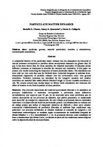
States and globally. PM10 and PM2.5 are criteria pollutants for which EPA has established national ambient air quality standards (NAAQS) to regulate concentrations and minimize health impacts. The 24 h NAAQS for PM10 and PM2.5 are currently 150 µg m−3 and 35 µg m−3 , respectively [4]. In order to ensure these standards are met, instruments that collect data for regulatory purposes must be certified as meeting rigorous quality standards. The EPA designates instruments that have met these standards as federal reference methods or federal equivalent methods (FRM, FEM). The beta attenuation monitor (BAM-1020, Met One Instruments Inc., Grant Pass, OR, USA) has been certified as an EPA FEM instrument for PM2.5 and PM10 , provided it is installed, operated, and calibrated according to established procedures. Air pollution has become a major concern for the public, as air pollution has received increased media attention, and local and national governments continue to publicize their efforts to improve air quality. Governments and other organizations are also broadcasting air quality data in real time, which has increased public awareness. The interest and demand for air quality data has led companies to develop low-cost portable air quality sensors. Some of these sensors are marketed directly to consumers who are interested in their personal exposure. The sensors also have a wide range of potential applications, depending on the quality of the measurements. Because the regulatory monitoring network maintained by the EPA is sparse, with a limited spatial density, low-cost sensors have the potential to provide insight into the spatial and temporal variability of pollutants; data from these sensors could inform studies of personal exposure and emission inventories if the quality of the measurement is robust enough to meet the given objectives [5,6]. Air quality researchers are also examining the deployment of sensor networks and the potential value of integrating these sensors into the existing air quality regulatory network [7,8]. However, different interpretations of data require different levels of confidence in data quality. The proliferation of measurements from low-cost air sensors presents data interpretation challenges, as few studies have examined the performance (i.e., accuracy, precision, and reliability) of the sensors under real-world conditions [6]. Quantifying the performance of low-cost air quality sensors is an active area of research, as studies examine sensor measurements in a variety of real-world environments and controlled conditions [9–11]. Studies have also examined the performance of a network of sensors, and the use of those measurements to quantify pollution hot spots [12,13]. The validity and uncertainty of sensor measurements over a range of different meteorological and aerosol loading environments needs to be quantified. The need to validate sensor measurements against established methods in real-world environments is key, as laboratory experiments do not typically reflect the variability of meteorological and pollution conditions found in the real world [11,14]. This is a requisite step to ensuring that sensors can be deployed for objectives appropriate to confidence in data quality. Santa Barbara County Air Pollution Control District (SBCAPCD) entered into contract with Sonoma Technology, Inc. (STI) to investigate the use of low-cost sensors for monitoring dust by conducting a pilot field study at Cuyama Valley High School in New Cuyama, California. This study evaluated the performance of two low-cost portable PM sensor models: the Optical Particle Counter, OPC-N2 (available for ~450 USD, Alphasense Ltd., Essex, UK) and the AirBeam (available for ~250 USD, HabitatMap Inc., Brooklyn, New York, NY, USA), for detecting particulate matter in the Cuyama Valley of California. Cuyama Valley is a sparsely populated area in southern California, with significant agriculture in the regions of the valley where the topography is flat. Figure 1 shows the general area of the Cuyama Valley and the location of the monitoring site at Cuyama Valley High School in relation to nearby agricultural areas. Major sources of particulate matter include wind-blown dust and regional transport. To examine regional transport patterns, STI modeled transport trajectories for several of the high PM10 concentration days identified during this study using the hybrid single-particle Lagrangian integrated trajectory (HYSPLIT) model. Modeled regional transport patterns suggest that, on some days, PM10 from the California Central Valley is transported to the New Cuyama area, contributing to the concentrations observed. However, the short-duration
Sensors 2017, 17, 1805
3 of 16
Sensors 2017, 17, 1805
3 of 16
high-concentration high-concentration events events reported reported by by the the sensors sensors suggest suggest that that local local transport transport of of dust dust is is also also aa major major contributor to the observed higher PM concentrations. contributor to the observed higher PM10 10 concentrations.
Figure 1. The location of Cuyama Valley in California (a), and the location of the field site within Figure 1. The location of Cuyama Valley in California (a); and the location of the field site within Cuyama Valley (b). Cuyama Valley (b).
The objectives of the study were to determine whether the low-cost PM sensors detect dust The objectives of well the study were to determine whether the low-cost PM sensors detect dust events events and if so, how they detect dust events; to determine how precise the sensor measurements and so, how well sensor they detect dust events; to determine precise sensor measurements and are, ifand whether precision is sufficient either how for use in athe network to monitor theare, spatial whether sensor precision is sufficient either for use in a network to monitor the spatial variability of PM, variability of PM, or to obtain localized data to augment information available from the regional or to obtain localized to augmentwhether information from thecontinuously regional monitoring network; monitoring network; data to determine the available sensors operate and meet data to determine whether the sensors operate continuously and meet data completeness requirements for completeness requirements for reliably detecting dust events; and to determine whether the sensors reliably detecting dust events; and to determine whether the sensors could be used as part of an “early could be used as part of an “early warning system” to inform decisions to reduce exposure to high warning system” to inform decisions to reduce exposure to high PM concentrations. PM concentrations. Precision was examined examinedby bycomparing comparingdata data from three sensors of the same model. Accuracy Precision was from three sensors of the same model. Accuracy was was examined by comparing sensor measurements with the FEM BAM, and with the GRIMM 11-R examined by comparing sensor measurements with the FEM BAM, and with the GRIMM 11-R optical optical (GRIMM Aerosol Technik GmbH & Co., Ainring,Germany). Germany).The Theimpact impact of particleparticle countercounter (GRIMM Aerosol Technik GmbH & Co., Ainring, of meteorology and the variations of the size distribution were also examined. The potential use these meteorology and the variations of the size distribution were also examined. The potential use of of these sensors sensors to to inform inform behavior behavior is is presented, presented, such such as as using using high high temporal temporal resolution resolution to to limit limit exposure. exposure. 2. Methodology 2. Methodology STI (Petaluma, CA, USA) deployed six low-cost PM sensor devices and conducted a three-month STI (Petaluma, CA, USA) deployed six low-cost PM sensor devices and conducted a three-month field study from 14 April 2016, to 6 July 2016, to characterize the performance of the sensors for field study from 14 April 2016, to 6 July 2016, to characterize the performance of the sensors for detecting PM events in the Cuyama Valley environment. Three OPC-N2 and three AirBeam sensors detecting PM events in the Cuyama Valley environment. Three OPC-N2 and three AirBeam sensors were deployed at Cuyama Valley High School to evaluate sensor performance over a range of were deployed at Cuyama Valley High School to evaluate sensor performance over a range of conditions. The sensors were collocated with a BAM-1020 measuring PM10 , a GRIMM 11-R measuring conditions. The sensors were collocated with a BAM-1020 measuring PM10, a GRIMM 11-R measuring particle sizes, and an R.M. Young 05305V meteorological station measuring wind speed and direction particle sizes, and an R.M. Young 05305V meteorological station measuring wind speed and direction at 1 min temporal resolution. The BAM-1020 was deployed to evaluate the accuracy of the OPC-N2 at 1 min temporal resolution. The BAM-1020 was deployed to evaluate the accuracy of the OPC-N2 PM10 measurements. Three of each of the two low-cost sensor models were deployed to assess sensor PM10 measurements. Three of each of the two low-cost sensor models were deployed to assess sensor precision and reliability. The GRIMM 11-R was deployed to obtain particle size information and assist precision and reliability. The GRIMM 11-R was deployed to obtain particle size information and assist with interpretation of sensor performance as a function of particle size. GRIMM 11-R measurements with interpretation of sensor performance as a function of particle size. GRIMM 11-R measurements of the particle size distribution were converted to particle mass distribution, including PM1 , PM2.5 , of the particle size distribution were converted to particle mass distribution, including PM1, PM2.5, and PM10 . and PM10. All of the instruments were collocated within a few feet of one another. Initially, three containers All of the instruments were collocated within a few feet of one another. Initially, three containers on a small tripod housed one OPC-N2 and one AirBeam sensor each. Each container was equipped with on a small tripod housed one OPC-N2 and one AirBeam sensor each. Each container was equipped with a vent to allow air to be drawn in and a small exhaust fan to blow air out. The meteorological equipment was located on a second tripod. The BAM and GRIMM 11-R were housed nearby in a
Sensors 2017, 17, 1805
4 of 16
a vent to allow air to be drawn in and a small exhaust fan to blow air out. The meteorological equipment was located on a second tripod. The BAM and GRIMM 11-R were housed nearby in a climate-controlled shelter. Data collected during the study were stored onsite and transmitted in real time to STI’s servers via a cellular modem for archival within a data management system developed for the project. To assess the impacts from sampling orientation on sensor measurements, the sampling orientation for the sensors was varied as shown in Table 1. The reference instruments, BAM and GRIMM 11-R, were oriented with omnidirectional sampling. On 1 June 2016, OPC-N2 A was relocated to a third tripod so that it could sample omni-directionally to assess the impacts of sampling orientation. Table 1. Instrument sampling orientation. Instrument
Sampling Orientation
BAM-1020 GRIMM 11-R OPC-N2 A OPC-N2 B OPC-N2 C AirBeam A AirBeam B AirBeam C
Omnidirectional Omnidirectional North/Omnidirectional * North South North North South
* Between 4 April 2016, and 1 June 2016, OPC-N2 A sampled from the north. On 1 June 2016, OPC-N2 A was relocated to a new tripod, where it sampled omnidirectionally until 6 July 2016.
Both the AirBeam and the OPC-N2 are optical particle counters (OPCs). An OPC measures the scattered light from a sampled stream of aerosol particles to reconstruct particulate mass concentration [15]. The AirBeam followed an open source development model, so the firmware and the electronic schematics for the instrument are available online. A light-emitting diode (LED) source of visible green light is used to detect particles, and the raw measurement provides particle counts for all particle sizes sampled. In this study, the default conversion algorithm was used to convert these counts (recorded in hundreds of particles per cubic feet, hppcf) to PM2.5 mass concentration at a one-minute temporal resolution, which includes assumptions about the particle mass density, refractive index of the particle, and the size distribution. This conversion factor is PM2.5 (µg·m−3 ) = 0.518 + 0.00274 × particle count (hppcf). The AirBeam sensor system also measures temperature and relative humidity [16]. The OPC-N2 uses a laser beam at 658 nm as the light source. The resulting scattered light is focused using an elliptical mirror toward a dual-element photodetector. The firmware of the OPC-N2 is considered proprietary information and includes default settings of 1.5 + 0i for the refractive index of particles and 1.65 g·cm−3 for particle mass density. The refractive index assumption is required because both the intensity and angular distribution of scattered light from the particle are dependent upon it. The OPC-N2 detects particles with diameters within the range of 0.38 µm to 17 µm. Each particle count is classified into one of 16 size bins within this range, resulting in an approximation of the particle size distribution. The firmware calculates values of PM1 , PM2.5 , and PM10 at a one-minute temporal resolution based on the particle size distribution using the assumed particle mass density value. The OPC-N2 is calibrated by the manufacturer using polystyrene spherical latex particles with a known diameter, refractive index, and density. No correction factor for particle density was applied to the data collected during this study. The assumed particle density of 1.65 g cm−3 may be a source of uncertainty for different chemical compositions of PM [17]. PM concentrations were also derived from a GRIMM 11-R OPC. The GRIMM 11-R also measures the particle size distribution through the detection of scattered light. The GRIMM 11-R classifies particle counts into 31 size bins between 0.25 µm and 32 µm at a one-minute resolution. The GRIMM 11-R instrument was designed for the detection of dust particles, which are a major source of PM in the Cuyama Valley environment. Therefore, it is possible that the GRIMM 11-R makes more accurate assumptions of the particle refractive index and in the scattering response of particles than
Sensors 2017, 17, 1805
5 of 16
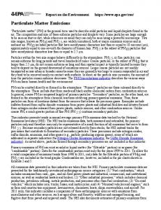
the OPC-N2 and the AirBeam. Concentrations of PM1 , PM2.5 , and PM10 were computed by converting the particle size distributions into particle volume distributions, using the center of the size bin as the particle diameter for all counts within each respective bin. Then, the total particle volume was computed by summing over the desired size range. A particle density of 1 g·cm−3 was used to convert the measurements to PM concentration values [18]. A BAM-1020 was deployed as a reference instrument to measure PM10 . The BAM-1020 is a designated EPA FEM for hourly PM10 monitoring and is used for over 80% of PM10 measurements in the United States at the federal, state, and local levels [19]. Particles larger than 10 µm in diameter are removed by a cyclone, and air is then passed through a chamber that is heated to 20 ◦ C before particles are impacted onto a filter tape that, after a period of collection, is exposed to a source of beta radiation [20]. The degree of absorption of that radiation by particulate matter collected on the filter tape is a sensitive measure of particle mass that is quantified by careful calibration procedures [20,21]. Because the instruments use different techniques and have different assumptions in their retrieval of PM values, there are known biases in their measurements depending on the size distribution and chemical composition of the aerosol particles. Because the OPC sensors rely on the detection of scattered light, the measurement of aerosols that are highly absorptive would have a significant low bias. This would be important in environments where the emission of incomplete combustion products leads to a high mass fraction of black carbon in PM. A recent study quantified this impact, showing that OPC-N2-measured values of PM2.5 and PM10 were a factor of 10 lower for highly absorptive welding fume aerosols than for salt aerosols, compared to the reference measurements by a scanning mobility particle sizer (SMPS) and an aerodynamic particle scanner (APS) [22]. This bias is not likely to be significant in an environment such as Cuyama Valley, where non-absorbing wind-blown dust is a major source of particulate matter. Another source of bias is the variability of the size distribution of the aerosols. Because the GRIMM 11-R has almost twice the size bin resolution as the OPC-N2, we can expect greater accuracy due to the variability in the size resolution. Further, the OPC-N2 would have greater accuracy than the AirBeam due to this bias, because the AirBeam converts particle counts to PM2.5 from one size bin of measurements while assuming a predetermined particle size distribution. GRIMM 11-R measurements are used to quantify how the varying particle size distribution can impact sensor measurements of PM. 3. Results and Discussion 3.1. Cuyama Aerosol Environment The wind rose of the full study period in Figure 2 shows low wind speeds (less than 2 m/s) from the southeast or low-to-moderate winds from the northwest the vast majority of the time. Figure 3 shows the hourly PM10 concentrations measured by the BAM. Daily average BAM PM10 measurements exceeded the threshold of 50 µg·m−3 on 18 out of 84 days (21% of the time). These high PM events, which, for hourly readings, sometimes exceeded 150 µg·m−3 , were typically short-term events during low wind speed conditions when winds were from the southeast. Examination of the back-trajectories during high PM periods using the HYSPLIT model showed that some high PM periods correlated with transport from the California Central Valley. This indicates that both wind-blown dust and regional transport contribute to high PM concentrations. High PM events also tend to happen at night or during the early morning in connection with local meteorology and transport patterns.
Sensors 2017, 17, 1805 Sensors 2017, 17, 1805 Sensors 2017, 17, 1805
6 of 16 6 of 16 6 of 16
Figure 2. Wind rose for the full study period: 14 April 2016, to 6 July 2016. Figure 2. Wind rose for the full study period: 14 April 2016, to 6 July 2016. Figure 2. Wind rose for the full study period: 14 April 2016 to 6 July 2016.
Figure 3. Hourly PM10 concentrations measured by the beta attenuation monitor (BAM)-1020 from Figure 3. Hourly PM10 concentrations measured by the beta attenuation monitor (BAM)-1020 from 14 14 April3.2016 to 6PM July10 2016. Figure Hourly concentrations measured by the beta attenuation monitor (BAM)-1020 from 14 April 2016, to 6 July 2016. April 2016, to 6 July 2016.
Sensors 2017, 17, 1805 Sensors 2017, 17, 1805
7 of 16 7 of 16
Precision 3.2. 3.2. Precision precision the instruments was evaluated by computing the linear TheThe precision of theof instruments was evaluated by computing the linear regression andregression correlationand correlation of two of the same instruments. The results, summarized in Table 2, are derived from of two of the same instruments. The results, summarized in Table 2, are derived from hourly hourly measurements of PM 2.5 from the AirBeam and PM10 from the OPC-N2. measurements of PM from the AirBeam and PM from the OPC-N2. 2.5
10
Table 2. Correlation linear regression of sensor measurements. Table 2. Correlation and and linear regression of sensor measurements. X Axis Instrument Y Axis Instrument R2 X Axis Y Axis AirBeam A AirBeam B 0.99 2 R Instrument Instrument AirBeam A AirBeam C 0.98 AirBeam AirBeam C AirBeam A B AirBeam B 0.990.95 OPC-N2 OPC-N2 B AirBeam A A AirBeam C 0.980.84 OPC-N2 A OPC-N2 B AirBeam B AirBeam C 0.950.81 OPC-N2 A OPC-N2 B OPC-N2 A OPC-N2 B 0.840.91 OPC-N2 OPC-N2 C OPC-N2 A A OPC-N2 B 0.810.85 OPC-N2 B OPC-N2 C 0.79
Linear Regression Linear y = 0.96x + 0.55 yRegression = 0.85x – 0.28 0.87x –+0.62 yy== 0.96x 0.55 y = 0.71x +–3.54 y = 0.85x 0.28 1.00x +–1.95 yy== 0.87x 0.62 y = 0.66x +3.45 y = 0.71x + 3.54 0.57x ++1.72 yy== 1.00x 1.95 y = 0.78x − 0.82
Number of Measurements Time Period Number of 1995 full Time Period Measurements 1995 full 19951998 full full 19951647 full full 842 14 April–1 June 1998 full 805 1 June–7 July 1647 full full 8421629 14 April–1 June 1725 full
OPC-N2 A OPC-N2 B 0.91 y = 0.66x + 3.45 805 1 June–7 July OPC-N2 A OPC-N2 C 0.85 y = 0.57x + 1.72 1629 full TheBAirBeams demonstrate a 0.79 very highyprecision throughout the study OPC-N2 OPC-N2 C = 0.78x −consistently 0.82 1725 fullperiod, over
a range of different meteorological conditions and over a range of different aerosol property conditions (chemical composition size distribution). The close to one-to-one linear regression The AirBeams demonstrate a veryand high precision consistently throughout the study period, over of AirBeam A vs. AirBeam B shown in Figure 4 is partially due to the fact that they are sampling in the a range of different meteorological conditions and over a range of different aerosol property conditions same direction (north) throughout the study. Although AirBeam C is oriented toward the south, (chemical composition and size distribution). The close to one-to-one linear regression of AirBeam we stillAirBeam see a very high precision correlation and linear relationship. A vs. B shown in Figure 4 is partially due toregression the fact that they are sampling in the same direction (north) throughout the study. Although AirBeam C is oriented toward the south, we still see a very high precision correlation and linear regression relationship.
Figure 4. Correlation and linear regression of AirBeam A and AirBeam B PM2.5 measurements. Figure 4. Correlation and linear regression of AirBeam A and AirBeam B PM2.5 measurements.
Sensors 2017, 17, 1805
8 of 16
The correlation among OPC-N2s is lower than among the AirBeams. Because OPC-N2 PM10 is measuring over a large size range, the natural variability of larger aerosol particles contributes to a lower correlation of OPC-N2 results. It is more challenging to measure a larger range of aerosol particles sizes with high precision. The OPC-N2 instruments also demonstrate high precision, by correlation. The relationship between the magnitudes of measured PM10 also show good agreement, with major differences due to changes in sampling orientation. The large particles, in combination with the sampling orientation differences, are likely two major factors contributing to the range of linear regressions. The one-to-one correlation for OPC-N2 A and B is the highest for the 14 April to 1 June period, the only period when two OPC-N2 instruments were sampling from the same direction (north). 3.3. Accuracy Comparison to BAM The accuracy of the instruments was evaluated by computing the linear regression and correlation of each instrument with the BAM. Table 3 summarizes the results using hourly values, derived from BAM PM10 , AirBeam PM2.5 , and OPC-N2 PM10 . Table 3. Correlation and linear regression of sensor versus BAM PM measurements. X Axis Instrument
Y Axis Instrument
R2
Linear Regression
Number of Measurements
Time Period
BAM BAM BAM BAM BAM BAM BAM BAM
AirBeam A AirBeam B AirBeam C OPC-N2 A OPC-N2 A OPC-N2 A OPC-N2 B OPC-N2 C
0.25 0.21 0.33 0.76 0.53 0.81 0.67 0.61
y = 0.06x + 5.52 y = 0.05x + 5.98 y = 0.06x + 4.15 y = 0.22x + 1.76 y = 0.21x + 2.71 y = 0.23x + 0.32 y = 0.16x + 4.62 y = 0.13x + 2.47
1995 1997 1998 1764 939 825 1799 1776
full full full full 14 April–1 June 1 June–7 July full full
The AirBeams show a lower correlation and associated linear regression against the BAM than the OPC-N2 instruments, partially because the AirBeams are only measuring the PM2.5 fraction of PM10 . The OPC-N2 instruments show higher correlations with the BAM instruments. Figure 5 shows the comparison between BAM and OPC-N2 B-measured PM10 throughout the study period. The major factors contributing to the range of linear regressions and the correlation factors are the sampling orientation, the drift of the OPC-N2 instruments (discussed later), and assumptions built into the retrieval algorithm of the OPC-N2. It may be that a bias in the way the OPC-N2 instruments are sampling the size distribution contributes as well. These factors contribute to the OPC-N2 instruments reporting a small fraction of the BAM-measured PM10 (approximately 20%).
Sensors 2017, 17, 1805 Sensors 2017, 17, 1805
9 of 16 9 of 16
Figure 5. Correlation and regression of OPC-N2 B and BAM-measured PM10 . Figure 5. Correlation and regression of OPC-N2 B and BAM-measured PM10.
3.4.3.4. Sampling Orientation Sampling Orientation Sampling orientation is aismajor contributor to the OPC-N2andand AirBeam-derived correlations Sampling orientation a major contributor to the OPC-N2AirBeam-derived correlations andand linear regression shown above. Consider the OPC-N2 results shown in Table 2; when OPC-N2 A linear regression shown above. Consider the OPC-N2 results shown in Table 2; when OPC-N2 andABand are sampling in the same orientation (14 April to 1 June), the linear regression gives a one-to-one B are sampling in the same orientation (14 April to 1 June), the linear regression gives a onerelationship. After OPC-N2 A OPC-N2 shifts to an sampling (1 June to 7 July), the relationship to-one relationship. After A omnidirectional shifts to an omnidirectional sampling (1 June to 7 July), the changes, with OPC-N2 B reporting 66% of what OPC-N2 A reports. This demonstrates that directional relationship changes, with OPC-N2 B reporting 66% of what OPC-N2 A reports. This demonstrates sampling can lead to an underestimation of underestimation measured PM10 . The samplingPM orientation also contributes that directional sampling can lead to an of measured 10. The sampling orientation to the relationships. Because the BAM also samples alsoBAM-derived contributes toaccuracy the BAM-derived accuracy relationships. Because the omni-directionally, BAM also samples the omnichange of sampling from north to omni-directional for OPC-N2 A on 1 June increases the coefficient directionally, the change of sampling from north to omni-directional for OPC-N2 A on 1 of June 2 , correlation from 0.53 to 0.81. Therefore, it is likely that omni-directional sampling determination, R 2 increases the coefficient of determination, R , correlation from 0.53 to 0.81. Therefore, it is likely that greatly improves the sampling accuracy of the OPC-N2 instrument. Theseofeffects are also instrument. dependent on the size omni-directional greatly improves the accuracy the OPC-N2 These effects distribution of the aerosols and the wind direction and wind speed of the meteorological environment. are also dependent on the size distribution of the aerosols and the wind direction and wind speed of The correlations and linear regressions of GRIMM 11-R-derived values of PM10 , PM2.5 and PM1 the meteorological environment. versus the BAM and sensor are of shown in Table 4. Because the GRIMM The correlations andmeasurements linear regressions GRIMM 11-R-derived values of PM10, 11-R PM2.5shows and PM1 a high degree of correlation and accuracy compared to BAM measurements, can use11-R GRIMM versus the BAM and sensor measurements are shown in Table 4. Because thewe GRIMM shows a 11-R-derived PM values to evaluate the size dependence of OPC N-2 observations, and compare high degree of correlation and accuracy compared to BAM measurements, we can use GRIMMthe 11-Rrelative accuracy of the AirBeam and the the OPC-N2 for PM2.5 of observations. This comparison that,the derived PM values to evaluate size dependence OPC N-2 observations, andshows compare while the OPC-N2 reports fraction ofand PMthe has a fairly compared to the GRIMM 10 , itOPC-N2 relative accuracy of thea AirBeam for high PM2.5correlation observations. This comparison shows 11-R. By contrast, the correlation of OPC-N2-measured PM and PM compared to the GRIMM 11-R 2.5 a fairly1 high correlation compared that, while the OPC-N2 reports a fraction of PM10, it has to the is significantly lower, partially the because of the downward drift of OPC-N2 (discussed later). GRIMM 11-R. By contrast, correlation of OPC-N2-measured PM2.5 values and PM 1 compared to the TheGRIMM AirBeam11-R demonstrates a higher accuracy for PM over thedrift course of this study, 2.5 measurements is significantly lower, partially because of the downward of OPC-N2 values
(discussed later). The AirBeam demonstrates a higher accuracy for PM2.5 measurements over the
Sensors 2017, 17, 1805
10 of 16
Sensors 2017, 17, 1805
10 of 16
both in terms of its linear regression and correlation compared to GRIMM 11-R values, in spite of course of this study, both in terms of its linear regression and correlation compared to GRIMM 11-R having a simpler measurement technique that does not account for variations in size distribution. values, in spite of having a simpler measurement technique that does not account for variations in size distribution. Table 4. Correlation and linear regression of GRIMM 11-R versus sensor and BAM PM measurements. Table 4. Correlation and linear regression of GRIMM 11-R versus sensorLinear and BAM PM measurements. Number of X Axis Y Axis Pollutant R2 Regression Measurements Instrument Instrument X Axis Instrument Y Axis Instrument Pollutant R2 Linear Regression Number of Measurements GRIMM 11-R GRIMM 11-R GRIMM 11-R GRIMM 11-R GRIMM 11-R GRIMM 11-R GRIMM 11-R GRIMM 11-R GRIMM 11-R GRIMM 11-R GRIMM 11-R GRIMM 11-R GRIMM 11-R GRIMM 11-R GRIMM 11-R GRIMM 11-R GRIMM 11-R GRIMM 11-R GRIMM 11-R GRIMM 11-R GRIMM 11-R GRIMM 11-R GRIMM 11-R GRIMM 11-R GRIMM 11-R GRIMM 11-R
BAM BAM OPC-N2 OPC-N2 A A OPC-N2 OPC-N2 B B OPC-N2 OPC-N2 C C OPC-N2 OPC-N2 A A OPC-N2 OPC-N2 B B OPC-N2 OPC-N2 C C OPC-N2 OPC-N2 A A OPC-N2 OPC-N2 B B OPC-N2 OPC-N2 C C AirBeam AirBeam A A AirBeam AirBeam B B AirBeam AirBeam C C
PM PM 1010 PM PM 1010 PM PM 1010 PM PM 1010 PM 2.5 PM 2.5 PM 2.5 PM 2.5 PM PM2.52.5 PM1 PM 1 PM1 PM 1 PM1 PM 1 PM2.5 PM 2.5 PM2.5 PM 2.5 PM2.5 PM 2.5
0.91 0.84 0.81 0.81 0.43 0.41 0.40 0.39 0.45 0.38 0.66 0.62 0.71
0.91y = 0.86xy+ =6.52 0.86x + 6.52 0.84y = 0.20xy+ =2.83 0.20x + 2.83 0.81y = 0.14xy+ =5.36 0.14x + 5.36 0.81y = 0.12xy+ =2.84 0.12x + 2.84 0.43y = 0.15xy+ =1.92 0.15x + 1.92 0.41y = 0.16xy+ =3.51 0.16x + 3.51 0.40y = 0.13xy+ =1.99 0.13x + 1.99 0.39y = 0.28xy+ =0.29 0.28x + 0.29 0.45y = 0.41xy+ =2.08 0.41x + 2.08 0.38y = 0.28xy+ =0.97 0.28x + 0.97 0.66y = 0.40xy+ =4.33 0.40x + 4.33 0.62y = 0.36xy+ =4.91 0.36x + 4.91 0.71y = 0.37xy+ =3.13 0.37x + 3.13
1753 1526 1626 1594 1521 1625 1590 1417 1623 1475 1753 1755 1755
1753 1526 1626 1594 1521 1625 1590 1417 1623 1475 1753 1755 1755
3.5. Size Distribution 3.5. Size Distribution As the linear regressions from Tables 2 and 3 show, the OPC-N2 reported a fraction of the PM10 As the linear regressions from Tables 3 and 4 show, the OPC-N2 reported a fraction of the values compared to both the BAM and GRIMM 11-R-derived measurements. GRIMM 11-R PM10 values compared to both the BAM and GRIMM 11-R-derived measurements. GRIMM 11-R measurements of the size distribution provide an opportunity to examine the cause of this bias. measurements of the size distribution provide an opportunity to examine the cause of this bias. Figure 6 Figure 6 shows the GRIMM 11-R-derived mass distribution of the aerosol particles, which includes shows the GRIMM 11-R-derived mass distribution of the aerosol particles, which includes the relative the relative contribution to PM10, PM2.5 and PM1 from each of the size bins measured. Toward the contribution to PM10 , PM2.5 and PM1 from each of the size bins measured. Toward the later part of later part of the study period, the GRIMM 11-R-derived mass distribution shows a shift to greater the study period, the GRIMM 11-R-derived mass distribution shows a shift to greater contributions contributions from larger particles. This shows that the precision and accuracy relationships derived from larger particles. This shows that the precision and accuracy relationships derived previously previously are valid over a range of different aerosol size distributions. are valid over a range of different aerosol size distributions.
Figure 6. GRIMM 11-R-derived mass distribution over the course of the study. Figure 6. GRIMM 11-R-derived mass distribution over the course of the study.
Given these conditions, it is likely that the OPC-N2 sensors were biased low in their measurement Given these conditions, it is likely that the OPC-N2 sensors were biased low in their and assessment of the contribution of particles between the 2.5 µm and 10 µm size range to PM10 . measurement and assessment of the contribution of particles between the 2.5 µ m and 10 µ m size Figure 6 shows that the contribution of these particles to PM10 is significant, and the majority of range to PM10. Figure 6 shows that the contribution of these particles to PM10 is significant, and the measurements made by OPC-N2 sensors showed PM10 less than 50 µg·m−3 . One contribution−3to this majority of measurements made by OPC-N2 sensors showed PM10 less than 50 µ g∙m . One contribution to this bias is the greater size bin resolution of the GRIMM 11-R instrument, which
Sensors 2017, 17, 1805 Sensors 2017, 17, 1805
11 of 16 11 of 16
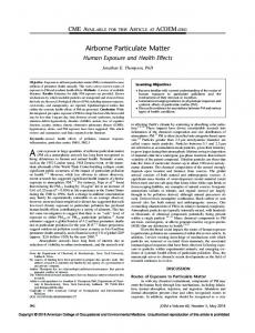
allows for more accurate particle sizing, and thus a more accurate assessment of the contribution of those particles to PM10. biasIn is the greater size bin of the 11-R instrument, which allows for more11-R accurate order to assess the resolution accuracy of the GRIMM sensors with respect to particle size, GRIMM PM particle sizing, and thus a more accurate assessment of the contribution of those particles to PM . concentrations were computed over a range of sizes. For each GRIMM 11-R size bin, the 10PM In order up to assess accuracy the sensors to particle 11-R concentration to and the including theofgiven size binwith was respect computed (PM0.25, size, PM0.27GRIMM , …, PM30 , PMPM 32, 2 concentrations were computed over a range of sizes. For each GRIMM 11-R size bin, the PM shown in the x axis of Figure 7). The R between each GRIMM 11-R PM concentration versus OPCconcentration the2.5given size bin was , . .analysis . , PM30 , 0.25 , PM N2 PM1, PM2.5, up PMto 10, and and including AirBeam PM concentrations arecomputed presented (PM in Figure 7.0.27 This 2 PM32 , shown x axis ofthe Figure The R between each GRIMM PM concentration versus presents a wayin ofthe examining size7). cut-off of the instruments, and the11-R accuracy of the instruments OPC-N2 PM , PM , PM , and AirBeam PM concentrations are presented in Figure 7. This analysis 1 varying 2.5 10 distribution over2.5 in sampling the size the course of the study. While the OPC-N2 PM10 shows presents a way of examining theatsize the range, instruments, and the accuracy of instruments the greatest absolute correlation thecut-off desiredofsize the highest correlations arethe with GRIMM in sampling the varying size distribution over the course of the study. While the OPC-N2 PM 10 shows 11-R PM3 and GRIMM 11-R PM6.5 and the range between them. The lower correlations between the the greatest absolute correlation at the desired size range, the highest correlations are with 6.5 µ m and 10 µ m size ranges indicate that the OPC-N2 was less accurate at sampling PM GRIMM greater 11-R6.5 PMµ3m, and GRIMM 11-R PMto6.5the and thefraction range between The lower correlations between the than which contributes low of PM10 them. that the OPC-N2 observes relative to the 6.5 µm and 10 µm size ranges indicate that the OPC-N2 was less accurate at sampling PM greater than GRIMM 11-R and the BAM (shown in Tables 2 and 3). While absolute OPC-N2 PM1 and PM2.5 6.5 µm, which to thetolow fraction of PM that the OPC-N2 observesaccurate relativecut-off to the GRIMM correlations arecontributes low compared GRIMM 11-R PM10ranges, they demonstrate sizing, 11-Rcorrelations and the BAM (shownatinorTables 3 and 4). While absolute OPC-N2 PM are 1 and 2.52correlations with peaking near the corresponding size bin at 1 µ m for PM1PM and µ m for PM2.5 . low compared to GRIMM 11-R PM ranges, they demonstrate accurate cut-off sizing, with correlations The AirBeam also shows an accurate size representation of PM2.5 compared to the GRIMM11-R, with peaking at or near the size bin at 1 µm for PM1 and 2 µm for PM2.5 . The AirBeam correlations peaking at 2corresponding µ m. also shows an accurate size representation of PM2.5 compared to the GRIMM11-R, with correlations peaking at 2 µm.
Figure 7. Coefficient of determination (R2 ) of OPC-N2 PM1 , PM2.5 , PM10 , AirBeam PM2.5 and GRIMM Figure 7. Coefficient of determination (R2) of OPC-N2 PM1, PM2.5, PM10, AirBeam PM2.5 and GRIMM 11-R-derived PM over a range of size ranges (PM from zero to size). 11-R-derived PM over a range of size ranges (PM from zero to size).
3.6.Meteorology Meteorologyand andSize SizeDistribution DistributionInfluence Influence 3.6. Figure 8 8 shows showsthetheAirBeam-measured AirBeam-measured GRIMM 11-R-derived 2.5 and 2.5 . Figure PMPM 2.5 and the the GRIMM 11-R-derived PM2.5. PM The The relationship between AirBeam and GRIMM 11-R-measured PM is a linear response, with 2.5 relationship between AirBeam and GRIMM 11-R-measured PM2.5 is a linear response, with a range values depending on the meteorology and variability aerosol characteristics, ofa range valuesof depending on the meteorology and variability of aerosolofcharacteristics, includingincluding aerosol aerosol chemical composition size distribution variability. In the right 8, color chemical composition and size and distribution variability. In the right panel of panel Figureof8,Figure color coding coding shows the average GRIMM particle size for the full range of GRIMM 11-R size bins. Large shows the average GRIMM particle size for the full range of GRIMM 11-R size bins. Large average average particle sizes lead to lower AirBeam PM measurements relative to the GRIMM 11-R. This 2.5 particle sizes lead to lower AirBeam PM2.5 measurements relative to the GRIMM 11-R. This reflects reflects the AirBeam measurement technique of detecting total particle scattering—with an assumed the AirBeam measurement technique of detecting total particle scattering—with an assumed size size distribution, the AirBeam has the possibility of underestimating or overestimating total PM2.52.5mass mass distribution, the AirBeam has the possibility of underestimating or overestimating total PM concentration.Figure Figure 88 provides provides evidence larger particles, AirBeams are concentration. evidence that, that,for forsize sizedistributions distributionswith with larger particles, AirBeams underestimating PM , and, conversely, AirBeams may be overestimating PM for size distributions 2.5 2.5 are underestimating PM2.5, and, conversely, AirBeams may be overestimating PM2.5 for size with smallerwith particles. However, one mechanism not be the of thedriver range distributions smaller particles.this However, this one may mechanism maydominant not be thedriver dominant values observed, as observed, the variability of variability the size distribution interdependent with meteorological ofofthe range of values as the of the sizeis distribution is interdependent with
Sensors 2017, 17, 1805 Sensors 2017, 17, 1805
12 of 16 12 of 16
meteorological conditions, chemical composition variability, and other mechanisms such as hygroscopic aerosol growth. In the left panel of Figure 8, the same AirBeam and GRIMM 11-R PM2.5 conditions, chemical composition variability, and other mechanisms such as hygroscopic aerosol values are color coded to show wind speed. For lower wind speeds, a trend toward lower AirBeam growth. In the left panel of Figure 8, the same AirBeam and GRIMM 11-R PM2.5 values are color coded values is observed, relative to the GRIMM 11-R. Other meteorological variables such as relative to show wind speed. For lower wind speeds, a trend toward lower AirBeam values is observed, relative humidity may also impact sensor accuracy. Figure 8 shows that both meteorological conditions and to the GRIMM 11-R. Other meteorological variables such as relative humidity may also impact sensor aerosol conditions can influence AirBeam measurements, and should be accounted for when sensor accuracy. Figure 8 shows that both meteorological conditions and aerosol conditions can influence measurements are calibrated with established standards. AirBeam measurements, and should be accounted for when sensor measurements are calibrated with established standards.
Figure 8. Comparison of GRIMM 11-R- and AirBeam-derived PM2.5 . Color coding shows wind Figure 8.(a) Comparison GRIMM 11-Rand size AirBeam-derived PM2.5. Color coding shows wind direction and GRIMMof11-R average particle (b). direction (a) and GRIMM 11-R average particle size (b).
3.7. Data Recovery 3.7. Data Recovery Table 5 summarizes data recovery from 14 April 2016, through 6 July 2016. Periods of data Table 5 summarizes recovery from (prior 14 April 2016, through July Periods of data loss loss that occurred during data system installation to 14 April 2016) 6are not2016. included in the number that occurred duringsince system installation (prior to 14 April 2016) are related not included the number of of of possible samples data loss during those periods was not to theinperformance possible samples since data loss during those periods was not related to the performance of the sensor the sensor technology. Data completeness of 75% of 1 min samples was required for each 1 h sample. technology. Data completeness of 75% of 188%) minon samples for eachtime 1 h frames sample.for Data Data completeness was high (greater than both 1 was min required and 1 h average all completeness was high (greater thanOPC-N2 88%) on data both during 1 min and h average frameswere for all sensors. sensors. Several periods of missing the1first half oftime the study caused by Several periods of missing OPC-N2 data during the first half of the study were caused by communication issues related to the data logger rather than the OPC-N2 sensor itself. Neglecting data communication issues to thedata datarecovery logger rather the OPC-N2 itself. loss related to the data related logger issue, for thethan OPC-N2 sensors sensor was over 99%Neglecting for 1-min data loss related to the data logger issue, data recovery for the OPC-N2 sensors was over 99% for data and approximately 100% for hourly data. 1-min data and approximately 100% for hourly data. Table 5. Data recovery for the sensors from 14 April 2016, through 6 July 2016. Table 5. Data recovery for the sensors from 14 April 2016, through 6 July 2016. Number of Number of Samples Sensor Number of Samples Recovered % Recovery % Recovery Sensor Number of Possible Samples % Recovery 1-min1-min% Recovery 1-h1-h Possible Samples Recovered
OPC-N2 A OPC-N2 A OPC-N2 B OPC-N2 B OPC-N2 C OPC-N2 C AirBeam A AirBeam B AirBeam A AirBeam C AirBeam B
120,181 120,181 120,181 120,181 120,181 120,181 120,181 120,181 120,181 120,181 120,181
105,934 *
88.1
88.7
105,934 * * 88.1 89.5 88.795.4 107,613 107,613 * * 89.5 88.3 95.492.4 106,204 106,204 * 88.3 99.5 92.4 119,548 100.0 119,689 100.0 119,548 99.5 99.6 100.0 119,689 100.0 119,689 99.6 99.6 100.0 AirBeam C 120,181 119,689 99.6 100.0 * Data recovery for the OPC-N2 was lower during the first half of the study due to an issue related to the data *communication Data recovery for with the OPC-N2 waslogger. lower during the first half of the study due to an issue related to communication with the data logger.
3.8. Drift of OPC-N2 Sensor 3.8. Drift of OPC-N2 Sensor All three OPC-N2 instruments demonstrated a gradual drift leading to lower PM measurements OPC-N2 instruments a gradual driftofleading to lower PM measurements over All the three course of the study. Figure 9demonstrated shows that over the course 12 weeks, the relationship between over the course of the study. Figure 9 shows that over the course of 12 weeks, the relationship between
Sensors Sensors2017, 2017,17, 17,1805 1805
13 13of of16 16
OPC-N2 B and BAM PM10 changes, with OPC-N2 B reporting 65% of its initial PM values toward the OPC-N2 B and BAM PM10 changes, with OPC-N2 B reporting 65% of its initial PM values toward end of the study. the end of the study.
Figure 9.9. Linear Linearregression regressionofofOPC-N2 OPC-N2B Bversus versus BAM PM forthe the first (green) and (blue) week Figure BAM PM for first (green) and lastlast (blue) week of 10 10 of the study. the study.
The drift drift was was quantified quantifiedin inaanumber numberof ofways: ways:the theOPC-N2 OPC-N2PM PM1010 values values were were compared compared against against The the BAM PM measurements and the GRIMM 11-R-derived PM 10 . OPC-N2 PM 2.5 values were the BAM PM measurements and the GRIMM 11-R-derived PM10 . OPC-N2 PM2.5 values were compared compared against GRIMM 11-R and PM2.5 values. In all cases, a consistent trend exists for against GRIMM 11-R and AirBeam PMAirBeam 2.5 values. In all cases, a consistent trend exists for the OPC-N2 the OPC-N2 measurements: a downward drift the the PMcourse valuesofover theweeks course of theto12 measurements: a downward drift of the PM valuesofover the 12 relative allweeks other relative to all other instruments. The AirBeam instruments do not demonstrate a drift in reported instruments. The AirBeam instruments do not demonstrate a drift in reported PM values, whichPM is values, which is confirmed by comparing AirBeam and GRIMM-derived PM2.5. confirmed by comparing AirBeam and GRIMM-derived PM2.5 . Onepossible possiblecause causeof of this this downward downwarddrift driftisisthe the buildup buildupof of dust dust on on the the fan, fan, which which would would impact impact One the flow rate through the sensor. This may be an acute challenge in the Cuyama Valley environment, the flow rate through the sensor. This may be an acute challenge in the Cuyama Valley environment, because of of the the long-term long-term presence presence of of dust dust events events with with high high particulate particulate concentrations concentrations and and large large dust dust because particles. The buildup of dust in the fan would lower the sampling efficiency of the OPC-N2, leading particles. The buildup of dust in the fan would lower the sampling efficiency of the OPC-N2, leading to aasmaller smallerfraction fraction of aerosols sampled be consistent with observed to of aerosols sampled over over time, time, whichwhich would would be consistent with observed OPC-N2 OPC-N2 performance in this study. Measuring the sample flow rate or routinely conducting performance in this study. Measuring the sample flow rate or routinely conducting maintenance of the maintenance the OPC-N2 flow system may help to this effect for future studies in dustOPC-N2 flow of system may help to alleviate this effect foralleviate future studies in dust-prone environments. prone environments. 3.9. Early Detection 3.9. Early Detection The one-minute resolution of the small sensors gives them the potential to be used as an early The one-minute resolution the small gives themaerosol the potential to be used as an early detection system for short termof events. Thesensors Cuyama Valley environment has significant detection system for short term events. The Cuyama the Valley aerosol has significant minute-to-minute variability. Figure 10 demonstrates ability of theenvironment OPC-N2 measurements to minute-to-minute Figure 10 demonstrates the ability its of hourly the OPC-N2 measurements to detect high aerosolvariability. loading events before the BAM has completed measurement. Because detect high aerosol loading events before the BAM has completed its hourly measurement. Because
Sensors 2017, 17, 1805 Sensors 2017, 17, 1805
14 of 16 14 of 16
the BAM samples the first 52 min of the hour, for a random distribution of short-term aerosol events, the BAM OPC-N2 instruments anhour, average detection time ofof 34short-term min. Because the BAM is the samples the firstwould 52 minhave of the for aearly random distribution aerosol events, not OPC-N2 measuring PM duringwould the last 8 min of the hour, OPC-N2time instruments has a 13% chance of the instruments have an average earlythe detection of 34 min. Because the BAM reporting a short-term aerosol event fails the to measure was observed in is not measuring PM during the last 8that minthe of BAM the hour, OPC-N2completely, instrumentsashas a 13% chance thereporting course ofathe study. aerosol event that the BAM fails to measure completely, as was observed of short-term in the course of the study.
Figure Figure 10. 10. Hourly Hourly PM PM10 10 concentrations concentrations measured measured by by the the BAM BAMand andone-minute one-minutePM PM1010 concentrations concentrations measured measuredby bythe the three three OPC-N2 OPC-N2sensors sensorson on10 10 June June 2016. 2016. The The BAM BAM measurements measurements at at 21:00 21:00 would would have have been been available available at at 22:00. 22:00.
4. 4. Conclusions Conclusions Having Having quantified quantifiedthe the performance performanceof of the the sensors, sensors, we we present present recommendations recommendations on on the the potential potential utility utility of of the the measurements measurements and and their deployment deployment in an environment like Cuyama Valley. Valley. In In Cuyama Cuyama Valley, Valley, there thereare areno noair airquality quality monitoring monitoring stations stations in in the the existing existing EPA EPA infrastructure; infrastructure; the the nearest nearest monitor Maricopa, approximately 20 km20to km the northeast. Cuyama Valley is a unique monitorisisin in Maricopa, approximately to the northeast. Cuyama Valley environment is a unique surrounded mountains,byand local air quality measurements could providecould valuable information environmentby surrounded mountains, and local air quality measurements provide valuable where none exists. sensors reported significantly measurements relative to the GRIMM information whereWhile none the exists. While the sensors reportedlow significantly low measurements relative 11-R and BAM (Tables 3 and 4), by a factor of 2–4, they be utilized as a still qualitative measure to the GRIMM 11-R and BAM (Tables 2 and 3), by a could factor still of 2–4, they could be utilized as a of high PM events. and instruments showed in reporting short-terminPM events. qualitative measureAll ofsensors high PM events. All sensors andcoherence instruments showed coherence reporting Furthermore, the sensors were routinely calibrated relative to a reference thea corrected short-term PMif events. Furthermore, if the sensors were routinely calibratedmonitor, relative to reference measurements would be more quantitative, calibration may need be carried may out monitor, the corrected measurements wouldalthough be more this quantitative, although thistocalibration periodically to compensate for the possible influence drift. need to be carried out periodically to compensate forof the possible influence of drift. The The low-cost low-cost sensors sensors demonstrate demonstrate aa robust robust quality quality of of performance performance by by certain certain measures, measures, such such as as high high precision precision and and reliability. reliability. The The OPC-N2 OPC-N2 and and the the AirBeam AirBeam showed showed high high precision precision over over aa range range of of conditions. each sensor model and PMPM variable) implies thatthat a seta conditions. The Thehigh highprecision precisionofofthe thesensors sensors(for (for each sensor model and variable) implies of can can be utilized to give a consistent, intercomparable measurement which is necessary for setsensors of sensors be utilized to give a consistent, intercomparable measurement which is necessary being deployed as a network. Sampling orientation was demonstrated to influence the accuracy of the for being deployed as a network. Sampling orientation was demonstrated to influence the accuracy measurements, which has implications for their for use their as personal orsensors instruments to be integrated of the measurements, which has implications use as sensors personal or instruments to be into networks. sampling would improve would the consistency PM measurements. integrated intoOmnidirectional networks. Omnidirectional sampling improveofthe consistency of PM The accuracy of the OPC-N2 is limited by its drift, which may be due to dust impacting measurements. the sampling flow rate. InOPC-N2 spite of this drawback, the OPC-N2 correlation The accuracy of the is limited by its drift, whichdemonstrates may be due reasonable to dust impacting the against the flow FEM standard BAM.ofThe low fraction ofthe PM10 measured by the OPC-N2 relative to the BAM sampling rate. In spite this drawback, OPC-N2 demonstrates reasonable correlation against the FEM standard BAM. The low fraction of PM10 measured by the OPC-N2 relative to the
Sensors 2017, 17, 1805
15 of 16
and GRIMM 11-R is likely due to a combination of drift, sampling of the size distribution, or an internal calibration to a different particle chemical composition/size distribution. The AirBeams demonstrated a higher degree of accuracy for measuring PM2.5 compared to GRIMM 11-R-derived PM2.5 (compared to the OPC-N2) in the Cuyama Valley environment. The one-minute time resolution of the sensors relative to the FEM monitors is an advantage. This could be used as an early warning detection system of PM events in Cuyama and in urban environments. This is a unique benefit in the environment of Cuyama Valley, where some high PM events are of very short duration, whereas the BAM reports hourly PM measurements, using the first 52 min of sampling. The sensors have demonstrated that they are useful for the assessment of short-term changes in the aerosol environment. Further examination of these emerging technologies is necessary, and sensors may be most useful as a supplement to the existing regulatory network. Incorporating collocation with established instruments in the field is encouraged for future studies. Acknowledgments: This work was partially funded by the Santa Barbara County Air Pollution Control District (SBCAPCD), Santa Barbara, CA, USA and SBCAPCD staff assisted with the study. We would like to thank SBCAPCD staff for helpful discussions throughout the study. Author Contributions: Anondo Mukherjee: Responsible for data quality control procedures, data analysis, data visualization, interpretation of results, and writing a majority of the manuscript text. Levi G. Stanton: Responsible for instrumental knowledge of sensors, field study design, data communication in the field, and assistance with interpretation of results and writing manuscript text. Ashley R. Graham: Assisted in interpretation of results and writing manuscript text. Paul T. Roberts: Assisted in interpretation of results and writing/reviewing manuscript text. Conflicts of Interest: The authors declare no conflict of interest. SBCAPCD staff assisted with the study.
References 1. 2. 3.
4. 5.
6. 7.
8.
9.
10.
Lelieveld, J.; Evans, J.S.; Fnais, M.; Giannadaki, D.; Pozzer, A. The contribution of outdoor air pollution sources to premature mortality on a global scale. Nature 2015, 525, 367–371. [CrossRef] [PubMed] World Health Organization. Ambient Air Pollution: A Global Assessment of Exposure and Burden of Disease; WHO Press: Geneva, Switzerland, 2016; pp. 23–37. ISBN 978-92-4-151135-3. Schlesinger, R.B.; Kunzli, N.; Hidy, G.M.; Gotschi, T.; Jerrett, M. The health relevance of ambient particulate matter characteristics: Coherence of toxicological and epidemiological inferences. Inhal. Toxicol. 2006, 18, 95–125. [CrossRef] [PubMed] EPA. NAAQS Table. Available online: https://www.epa.gov/criteria-air-pollutants/naaqs-table (accessed on 20 June 2017). Kumar, P.; Morawska, L.; Martani, C.; Biskos, G.; Neophytou, M.; Di Sabatino, S.; Bell, M.; Norford, L.; Britter, R. The rise of low-cost sensing for managing air pollution in cities. Environ. Int. 2015, 75, 199–205. [CrossRef] [PubMed] Lewis, A.; Edwards, P. Validate personal air-pollution sensors. Nature 2016, 535, 29–31. [CrossRef] [PubMed] Hall, E.S.; Kaushik, S.M.; Vanderpool, R.W.; Duvall, R.M.; Beaver, M.R.; Long, R.W.; Solomon, P.A. Integrating sensor monitoring technology into the current air pollution regulatory support paradigm: Practical considerations. Am. J. Environ. Eng. 2014, 4, 147–154. Jiao, W.; Hagler, G.; Williams, R.; Sharpe, R.; Brown, R.; Garver, D.; Judge, R.; Caudill, M.; Rickard, J.; Davis, M.; et al. Community Air Sensor Network (CAIRSENSE) project: Evaluation of low-cost sensor performance in a suburban environment in the southeastern United States. Atmos. Meas. Tech. 2016, 9, 5281–5292. [CrossRef] Snyder, E.G.; Watkins, T.H.; Solomon, P.A.; Thoma, E.D.; Williams, R.W.; Hagler, G.S.W.; Shelow, D.; Hindin, D.A.; Kilaru, V.J.; Preuss, P.W. The changing paradigm of air pollution monitoring. Environ. Sci. Technol. 2013, 47, 11369–11377. [CrossRef] [PubMed] Nieuwenhuijsen, M.J.; Donaire-Gonzalez, D.; Rivas, I.; de Castro, M.; Cirach, M.; Hoek, G.; Seto, E.; Jerrett, M.; Sunyer, J. Variability in and agreement between modeled and personal continuously measured black carbon levels using novel smartphone and sensor technologies. Environ. Sci. Technol. 2015, 49, 2977–2982. [CrossRef] [PubMed]
Sensors 2017, 17, 1805
11.
12. 13.
14.
15. 16. 17. 18. 19. 20.
21. 22.
16 of 16
Piedrahita, R.; Xiang, Y.; Masson, N.; Ortega, J.; Collier, A.; Jiang, Y.; Li, K.; Dick, R.P.; Lv, Q.; Hannigan, M.; Shang, L. The next generation of low-cost personal air quality sensors for quantitative exposure monitoring. Atmos. Meas. Tech. 2014, 7, 3325–3336. [CrossRef] Gao, M.; Cao, J.; Seto, E. A distributed network of low-cost continuous reading sensors to measure spatiotemporal variations of PM2.5 in Xi’an, China. Environ. Pollut. 2015, 199, 56–65. [CrossRef] [PubMed] Mead, M.I.; Popoola, O.A.M.; Stewart, G.B.; Landshoff, P.; Calleja, M.; Hayes, M.; Baldovi, J.J.; McLeod, M.W.; Hodgson, T.F.; Dicks, J.; et al. The use of electrochemical sensors for monitoring urban air quality in low-cost, high-density networks. Atmos. Environ. 2013, 70, 186–203. [CrossRef] Jovaševi´c-Stojanovi´c, M.; Bartonova, A.; Topalovi´c, D.; Lazovi´c, I.; Pokri´c, B.; Ristovski, Z. On the use of small and cheaper sensors and devices for indicative citizen-based monitoring of respirable particulate matter. Environ. Pollut. 2015, 206, 696–704. [CrossRef] [PubMed] Hinds, W.C. Aerosol Technology: Properties, Behavior, and Measurement of Airborne Particles, 2nd ed.; Wiley-Interscience: New York, NY, USA, 1999; ISBN 978-0-471-19410-1. Aircasting. Available online: http://aircasting.org/about (accessed on 15 May 2017). Alphasense Ltd. User Manual: OPC-N2 Optical Particle Counter. 072–0300, Issue 3; Alphasense Ltd.: Braintree, UK, 2015. GRIMM Aerosol Technik GmbH & Co. GRIMM Portable Aerosol Spectrometer, Datasheet. 11-R; GRIMM Aerosol Technik GmbH & Co. KG: Ainring, Germany, 2016. EPA. List of Designated Reference and Equivalent Methods. Available online: https://www3.epa.gov/ ttnamti1/files/ambient/criteria/AMTIC%20List%20Dec%202016-2.pdf (accessed on 20 June 2017). EPA. Standard Operating Procedure for the Continuous Measurement of Particulate Matter. Available online: https://www3.epa.gov/ttnamti1/files/ambient/pm25/sop_project/905505_BAM_SOP_Draft_ Final_Oct09.pdf (accessed on 20 June 2017). Castellani, B.; Morini, E.; Filipponi, M.; Nicolini, A.; Palombo, M.; Cotana, F.; Rossi, F. Comparative analysis of monitoring devices for particulate content in exhaust gases. Sustainability 2014, 6, 4287–4307. [CrossRef] Sousan, S.; Koehler, K.; Hallett, L.; Peters, T.M. Evaluation of the Alphasense optical particle counter (OPC-N2) and the Grimm portable aerosol spectrometer (PAS-1.108). Aerosol Sci. Technol. 2016, 50, 1–14. [CrossRef] © 2017 by the authors. Licensee MDPI, Basel, Switzerland. This article is an open access article distributed under the terms and conditions of the Creative Commons Attribution (CC BY) license (http://creativecommons.org/licenses/by/4.0/).