Assessment of Bayesian network classifiers as tools for ... - Lania

Assessment of Bayesian network classifiers as tools for discriminating breast cancer pre-diagnosis based on three diagnostic methods Ameca-Alducin Mar´ıa Yaneli1 , Cruz-Ram´ırez Nicandro2 , Mezura-Montes Efr´en1 , Martin-Del-Campo-Mena Enrique3 , P´erez-Castro Nancy1 , and Acosta-Mesa H´ector Gabriel2 1

Laboratorio Nacional de Inform´ atica Avanzada (LANIA) A.C. R´ebsamen 80, Centro, Xalapa, Veracruz, 91000, M´exico 2 Departamento de Inteligencia Artificial, Universidad Veracruzana Sebasti´ an Camacho 5, Centro, Xalapa, Veracruz, 91000, M´exico 3 Centro Estatal de Cancerolog´ıa: Miguel Dorantes Mesa Aguascalientes 100, Progreso Macuiltepetl,Xalapa, Veracruz, 91130, M´exico

August 25, 2012

Abstract. In recent years, a technique known as thermography has been again seriously considered as a complementary tool for the pre-diagnosis of breast cancer. In this paper, we explore the predictive value of thermographic atributes, from a database containing 98 cases of patients with suspicion of having breast cancer, using Bayesian networks. Each patient has corresponding results for different diagnostic tests: mammography, thermography and biopsy. Our results suggest that these atributes are not enough for producing good results in the pre-diagnosis of breast cancer. On the other hand, these models show unexpected interactions among the thermographical attributes, especially those directly related to the class variable. Keywords: Thermography

1

Breast cancer

Bayesian networks

Introduction

Nowadays, breast cancer is the first cause of death among women worldwide [1]. There are various techniques to pre-diagnose this disease such as autoexploration, mammography, ultrasound, MRI and thermography [2–5]. The commonest test for carrying out this pre-diagnosis is mammography [2]; however, due to the different varieties of such disease [3], there are situations where this test does not provide an accurate result [6]. For instance, women younger than 40-years old have more density in their breast: this is an identified cause for mammography not to work properly [7]. In order to overcome this limitation in the pre-diagnosis of breast cancer, a relatively new technique has been proposed as

a complement in such pre-diagnosis: thermography [5]. Such technique consists of taking infrared images of the breasts with an infrared camera [8]. Thermography represents a non-invasive, painless procedure, which does not expose to the patient to x-ray radiation [7]. Besides, it is cheaper than other pre-diagnostic procedures. Thermography gives mainly information about temperature of the breasts and their corresponding differences. It is argued that lesions in the breasts produce significantly more temperature than healthy, normal breasts [9]. This is because these lesions (or tumors) contain more veins and a have metabolic rate than the surrounding tissue. Our main contribution is the exploration of the predictive value of the atributes for three different diagnostic methods for breast cancer. With this exploration, we can more easily appreciate the performance of each method regarding accuracy, sensitivity and specificity. Moreover, we can visually identify which thermographic variables are considered, from the point of view of a Bayesian network, more important to predict the outcome. The rest of the paper is organized as follows. Section 2 describes the state of the art that gives the proper context so that our contribution is more easily identified. Section 3 presents the materials and methods used in our experiments. Section 4 presents the methodology to carry out such experiments and the respective results. Section 5 discusses these results and, finally, section 6 gives the conclusions and identifies some future work.

2

State of the Art

The state of the art of thermography includes introductory investigations, imagebased works and data-based works [10, 11]. The first ones focus on the explanation of the technique as well as its advantages and disadvantages. A representative work is that of Foster (1998) [6], who points out that thermography may be a potential alternative diagnostic method since it does not produce radiation. The second ones concentrate on techniques for image processing such as clustering or fractal analyses[12, 13]. The work of EtehadTavakol et al. (2008) [12] uses k-means and fuzzy c-means for separating lesions from no-lesions. The final ones present statistical and Artificial Intelligence techniques (such as Artificial Neural Networks) [14, 15, 7, 16]. The work of Wishart et al. (2010) [16] performs the comparison between two software that uses AI techniques for analyzing data coming from thermographic images so that diagnosses can be carried out. Our work focuses on the exploration of discriminative power of thermographic atributes for the pre-diagnosis of breast cancer using Bayesian networks.

3 3.1

Materials and Methods The Database

We used a 98-case database which was provided by a medical oncologist who specializes in the study thermographic since 2008. The database consists of 77

sick patients and 21 healthy patients. Each of the patients (either sick or healthy) has tests for thermography, mammography and biopsy. 28 variables in total form this dataset: 16 belong to thermography, 8 belong to mammography and 3 to biopsy; the last variable taken into account is outcome (cancer and no cancer). This last variable is confirmed by an open biopsy, which is considered as the gold-standard test for diagnosing breast cancer. Table 1 presents the names and a brief description of the corresponding thermographic variables. Table 2 presents the same information for mammographic variables while Table 3 for biopsy variables.

Table 1. Names, definitions and types of variables of thermography Variable name

Definition

Variable type

Asymmetry Degree difference (in Celsius) between the right and the left breasts Thermovascular network Amount of veins with highest temperature Curve pattern Heat area under the breast Hyperthermia Hottest point of the breast 2c Degree difference between the hottest points of the two breasts F unique Amount of hottest points 1c Hottest point in only one breast Furrow Furrows under the breasts Pinpoint Veins going to the hottest points of the breasts Hot center The center of the hottest area Irregular form Geometry of the hot center Histogram Histogram in form of a isosceles triangle Armpit Difference degree between the 2 armpits Breast profile Visually altered profile Score The sum of values of the previous 14 variables Age Age of patient Outcome Cancer/no cancer

Nominal Nominal Nominal Binary Nominal Nominal Binary Binary Binary Binary Binary Binary Binary Binary Binary Nominal Binary

(range [1-3]) (range [1-3]) (range [1-3]) (range [1-4]) (range [1-4])

(range [1-3])

Table 2. Names, definitions and types of variables of mammography Variable name

Definition

BIRADS Clockwise Visible tumor spiculated edges Irregular edges microcalcifications AsymmetryM distortion

Assigned value in a mammography to measure the degree of the lesion Nominal (range [0-6]) Clockwise location of the lesion Nominal (range [1-12]) Whether the tumor is visible in the mammography Binary Whether the edges of the lesion are spiculated Binary Whether the edges of the lesion are irregular Binary Whether microcalcifications are visible un the mammography Binary Whether the breast tissue is asymmetric Whether the structure of the breast is distorted Binary

Variable type

Table 3. Names, definitions and types of variables of biopsy Variable name Definition sizeD RHP SBRdegree

Variable type

Tama˜ no del tumor discretizado Nominal (range [1-3]) Types of cancer Nominal (range [1-8]) degree of cancer malignancy Nominal (range [0-3])

3.2

Bayesian Networks

A Bayesian network (BN) [17, 18] is a graphical model that represents relationships of probabilistic nature among variables of interest. Such networks consist of a qualitative part (structural model), which provides a visual representation of the interactions amid variables, and a quantitative part (set of local probability distributions), which permits probabilistic inference and numerically measures the impact of a variable or sets of variables on others. Both the qualitative and quantitative parts determine a unique joint probability distribution over the variables in a specific problem [17–19]. In other words, a Bayesian network is a directed acyclic graph consisting of [20]: a) nodes (circles), which represent random variables and arcs (arrows), which represent probabilistic relationships among these variables and for each node, there exists a local probability distribution attached to it, which depends on the state of its parents. Figures 1 and 2 (see section 4) show examples of a BN. One of the great advantages of this model is that it allows the representation of a joint probability distribution in a compact and economical way by making extensive use of conditional independence, as shown in equation 1: P (X1 , X2 , ..., Xn ) =

n Y

P (Xi |P a(Xi ))

(1)

i=1

Where P a(Xi ) represents the set of parent nodes of Xi ; i.e., nodes with arcs pointing to Xi . Equation 1 also shows how to recover a joint probability from a product of local conditional probability distributions. Bayesian Network Classifiers Classification refers to the task of assigning class labels to unlabeled instances. In such a task, given a set of unlabeled cases on the one hand, and a set of labels on the other, the problem to solve is to find a function that suitably maps each unlabeled instance to its corresponding label (class). As can be inferred, the central research interest in this specific area is the design of automatic classifiers that can estimate this function from data (in our case, we are using Bayesian networks). This kind of learning is known as supervised learning [21–23]. For the sake of brevity and the lack of space, we do not write here the code of the procedures used in the tests carried out in this work. Instead, we only describe them briefly and refer the reader to their original sources. The procedures used in these tests are: a) the Na¨ıve Bayes classifier, b) Hill-Climber and c) Repeated Hill-Climber [24, 25, 22]. a) The Na¨ıve Bayes classifier (NB) between are the main appeals are simplicity and accuracy: although its structure is always fixed (the class variable has an arc pointing to every attribute). In simple terms, the NB learns for maximum likelihood, from a training data sample, the conditional probability of each attribute given the class. Then, once a new case arrives, the NB uses Bayes’

rule to compute the conditional probability of the class given the set of attributes selecting the value of the class with the highest posterior probability. b) Hill-Climber is a Weka’s [24] implementation of a search and scoring algorithm, which uses greedy-hill climbing [26] for the search part and different metrics for the scoring part, such as BIC (Bayesian Information Criterion), BD (Bayesian Dirichlet), AIC (Akaike Information Criterion) and MDL (Minimum Description Length). For the experiments reported here, we selected the MDL metric. This procedure takes as input an empty graph and a database and applies different operators for building a Bayesian network: addition, deletion or reversal of an arc. In every search step, it looks for a structure that minimizes the MDL score. In every step, the MDL is calculated and procedure Hill-Climber keeps the structure with the best (minimum) score. It finishes searching when no new structure improves the MDL score of the previous network. c) Repeated Hill-Climber is a Weka’s [24] implementation of a search and scoring algorithm, which uses repeated runs of greedy-hill climbing [26] for the search part and different metrics for the scoring part, such as BIC, BD, AIC and MDL. For the experiments reported here, we selected the MDL metric. In contrast to the simple Hill-Climber algorithm, repeated Hill-Climber takes as input a randomly generated graph. It also takes a database and applies different operators (addition, deletion or reversal of an arc) and returns the best structure of the repeated runs of the Hill-Climber procedure. With this repetition of runs, it is possible to reduce the problem of getting stuck in a local minimum [19].

3.3

Evaluation Method: Stratified K-fold Cross-validation

We follow the definition of the cross-validation method given by Kohavi [23]. In k-fold cross-validation, we split the database D in k mutually exclusive random samples called the folds: D1 , D2 , . . . , Dk , where such folds have approximately equal size. We train this classifier each time i ∈ 1, 2, . . . , k using D \ Di and test it on Di (again, the symbol denotes set difference). The cross-validation accuracy estimation is the total number of correct classification divided by the sample size (total number of instances in D). Thus, the k-fold cross validation estimate is: acccv =

1 n

X

δ(I(D \ D(i) , vi ), yi )

(2)

(vi ,yi )∈D

Where (I(D \ D(i) , vi ), yi ) denotes the label assigned by classifier I to an unlabeled instance vi on dataset D \ D(i) (it means using the data set unless the test set), yi is the class of instance vi , n is the size of the complete dataset and δ(i, j) is a function where δ(i, j) = 1 if i = j and 0 if i 6= j. In other words,

if the label assigned by the inducer to the unlabeled instance vi coincides with class yi , then the result is 1; otherwise, the result is 0; i.e., we consider a 0/1 loss function in our calculations of equation 2. It is important to mention that in stratified k-fold cross-validation, the folds approximately contain (roughly) the same proportion of classes as in the complete dataset D. A special case of cross-validation occurs when k = n (where n represents the sample size). This case is known as leave-one-out cross-validation [21, 23]. For differents classifier, we assess the performance of the classifiers presented in section 3.2 using the following measures [27–30]: a) Accuracy: the overall number of correct classifications divided by the size of the corresponding test set. b) Sensitivity: the ability to correctly identify those patients who actually have the disease. c) Specificity: the ability to correctly identify those patients who do not have the disease

4

Methodology and Experimental Results

The procedure for making thermographic study begins with the obtaining the thermal images. These images are taken from 1 meter away of the patient, depending on her muscular mass in a temperature-controlled room (18-22o C), with a FLIR A40 infrared camera. Three images are taken for each patient: one frontal and two laterals (left and right). Right after, the breasts are uniformly covered with surgical spirit (using a cotton). Two minutes after, the same three images are taken again. All these images are stored using the ThermaCAM Researcher Professional 2.9 software. Once the images are taken and stored, the specialist analyzes them and fills in the database with the corresponding values for each thermographic variable. He also includes the corresponding values for mammographic and biopsy variables. We carried out the experiments using Weka [24], using the three different Bayesian network classifiers (see their parameter set in table 4) and other classifiers that were used in Weka are: Artificial Neural Network, decision tree ID3 and C4.5 (with default parameters). For measuring their accuracy, sensitivity and specificity, we used 10-fold cross-validation as described in section 3.3. The main objective of these experiments is to the exploration the diagnostic performance of the atributes of the thermography, mammography and biopsy, including the unveiling of the interactions among attributes and class. Table 5 shows the numerical results of thermography, mammography, biopsy and thermography and mammography for Na¨ıve Bayes, Hill-Climber and Repeated Hill-Climber. Table 6 shows the numerical results of thermography, mammography, biopsy and thermography and mammography for Artificial Neural Network, decision tree ID3 and tree C4.5. Figures 2- 7 show the BN corresponding to Hill-Climber and Repeated Hill-Climber for thermography, mammography and biopsy respectively. We do not present the structure of the Na¨ıve

Bayes classifier since its structure is always fixed: there is an arc pointing to every attribute from the class. Table 4. Used the following values for Hill-Climber and Repeated Hill-Climber Parameters

Hill-Climber

Repeated Hill-Climber

The initial structure NB (Na¨ ıve Bayes) Number of parents Runs Score type Seed arc reversal

False 100,000 MDL True

False 100,000 10 MDL 1 True

Table 5. Accuracy, sensitivity and specificity of Na¨ıve Bayes, Hill-Climber and Repeated Hill-Climber for different methods of pre-diagnosis of breast cancer. For the accuracy test, the standard deviation is shown next to the accuracy result. For the remaining tests, their respective 95% confidence intervals (CI) are shown in parentheses. Method

Na¨ ıve Bayes Accuracy Sensitivity

Thermography 68.18% (±12.15) Mammography 80.67% (±10.95) biopsy 99% (±3.16) Thermography 77.22% and mammog- (±14.13) raphy

HillClimber Specificity Accuracy Sensitivity

79%(70-88) 24%(6-42) 78.56% (±3.14) 87%(0-0) 52.4%(072.56% 0) (±10.30) 99%(80-95) 100%(100- 99% 100) (±3.16) 84%(76-93) 52%(3169.44% 74) (±10.37)

Repeated HillClimber Specificity Accuracy Sensitivity

100%(100- 0%(0-0) 100) 84%(76-93) 71%(5291) 84%(76-93) 100%(100100) 83%(75-91) 19%(2-36)

78.56% (±3.14) 74.56% (±8.26) 99% (±3.16) 70.56% (±11.85)

Specificity

100%(100- 0%(0-0) 100) 87%(80-95) 71%(5291) 87%(80-95) 100%(100100) 84%(76-93) 19%(2-36)

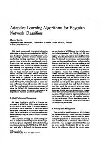
Fig. 1. Bayesian network resulting from running Hill-Climber and Repeated HillClimber with the biopsy 98-case database

Table 6. Accuracy, sensitivity and specificity of Artificial Neural Network, decision tree ID3 and C4.5 for different methods of pre-diagnosis of breast cancer. For the accuracy test, the standard deviation is shown next to the accuracy result. For the remaining tests, their respective 95% confidence intervals (CI) are shown in parentheses. Method

Artificial Neural Network Accuracy Sensitivity

Thermography 70.19% (±11.43) Mammography 85.30% (±9.55) biopsy 100% (±0) Thermography 76.11% and mammog- (±12.91) raphy

Decision Tree ID3 Specificity Accuracy Sensitivity

78%(69-87) 33%(1353) 92%(86-98) 67%(4787) 100%(100- 100%(100100) 100) 87%(80-95) 48%(2669)

74.87% (±12.15) *73.79% (±12.79) 97.33% (±5.75) 68.67% (±12.56)

Decision Tree C4.5 Specificity Accuracy Sensitivity

89%(82-96) 52%(3174) 94%(8861%(39100) 84) 100%(100- 100%(100100) 100) 76%(67-86) 41%(1865)

75.58% 94%(88-99) (±6.82) *77.96% 97%(94(±4.36) 101) 100%(±0) 100%(100100) 74.36% 94%(88-99) (±8.70)

Specificity 5%(-4-14) 0%(0-0) 100%(100100) 5%(-4-14)

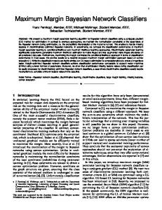
Fig. 2. Bayesian network resulting from running Hill-Climber with the thermographic 98-case database

Fig. 3. Bayesian network resulting from running Repeated Hill-Climber with the thermographic 98-case database

Fig. 4. Bayesian network resulting from running Hill-Climber with the mammography 98-case database

Fig. 5. Bayesian network resulting from running Repeated Hill-Climber with the mammography 98-case database

Fig. 6. Bayesian network resulting from running Hill-Climber with the thermographic and mammography 98-case database

Fig. 7. Bayesian network resulting from running Repeated Hill-Climber with the thermographic and mammography 98-case database

5

Discussion

Our main objective was explore the predictive value of thermographic atributes for pre-diagnosis of breast cancer. We decided to use the framework of Bayesian networks because its power to visually unveil the relationships among attributes themselves and among the attributes and the class. Furthermore, this model allows one to represent the uncertainty usually contained in the medical domain. First of all, let us check the accuracy, sensitivity and specificity performance of the Bayesian network classifiers using for the thermographic atributes (see Table 5). The results of Bayesian networks for thermography and mammography are almost comparable, but for the neural network (see table 6) mammography has an accuracy of 85.30%. In fact, thermography is excellent in identifying cases with the disease (100% sensitivity) but it performs very poorly for detecting healthy cases (0% specificity) for both Hill-Climber and Repeated Hill-Climber classifiers. And if we compare the results of the table 6 for Neural network, ID3 and C4.5, Bayesian classifiers (78.56%) obtained increased accuracy. As seen in the table 5. It is remarkable the change in the performance of these two pre-diagnosis techniques with the inclusion of all their respective variables (Na¨ıve Bayes classifier): 24% for thermography and 52.4% for mammography. It seems that this inclusion, far from improving the performance, makes it worse. Coming back to sensitivity and specificity values, it can be argued that in a certain sense, thermography can indeed be useful as a complementary tool for the pre-diagnosis of breast cancer. To see the picture more clearly, imagine a patient with a mammographic positive result for cancer. In order to be more certain of this result, a thermography can be taken to confirm it since thermography seems to identify without much trouble a sick patient. The biopsy (see results in the tables 5, 6) is indeed the gold-standard method to diagnose breast cancer. One question that immediately pops up is: why not then always use biopsy to diagnose breast cancer? The answer is because it implies a surgical procedure that involves known risks such as those that have mainly to do with anesthesia apart from the economical costs. Methods such as mammography try to minimize the number of patients undertaking surgery. In other words, if all non-surgical procedures fail in the diagnosis, biopsy is the ultimate resource. Regarding the unveiling of the relationships among attributes and among the attributes and the outcome, we can detect various interesting issues. For the case of thermography, contrary to what was expected, there is only one variable directly responsible for the explaining the behavior of the outcome: variable furrow (figures 2 and 3). It seems that this variable is enough for obtain the maximum percentage of classification (78.56%) for identifying patients with cancer. For the case of mammography, variables distortion and BIRADS are the only responsible to detect abnormal cases as well as normal cases (figures 4 and 3). This may mean that radiologists could just observe these two variables to diagnose the presence/absence of the disease. For the case of biopsy, we have more arguments to trust in this technique, in spite of its related and well-known risks.

Finally, Table 5 suggests not to analyze the thermographic and mammographic variables together but separated: the former decreases accuracy, sensitivity and specificity performance.

6

Conclusions and Future Work

Our results suggest that thermography may have potential as a tool for prediagnosing breast cancer. However, more study and tests are needed. Its overall accuracy and sensitivity values are encouraging; however, on the other hand, its specificity values are disappointed. The Bayesian networks, resultant from running 3 algorithms on the thermography database, give us a good clue for this behavior: it seems that most of thermographic variables are rather subjective, making it difficult to avoid the usual noise in this kind of variables. The present study allows then to think revisiting these variables and the way they are being measured. Such subjectivity does not belong only to thermography but also to mammography: according to the Bayesian network results, just two variables are responsible for explaining the outcome. Indeed, as can be noted from these results, when all mammographic variables are included (Na¨ıve Bayes classifier) the specificity values drop significantly with respect to those when only a subset of such attributes is considered. Moreover, if there were no subjectivity regarding specificity, then Na¨ıve Bayes would perform better. Thus, it seems that there exists an overspecialization of the expert radiologist in the sense of considering all variables for diagnosing patients with the disease but an underspecialization for diagnosing the absence of such a disease. It is important to mention that our database is unbalanced: we need to get more data (healthy and sick cases) so that our conclusions are more certain. For future work, we firstly propose to add more cases to our databases. Secondly, it would be desirable to have roughly the same number of positive and negative cases. Thirdly balancing classes. Finally, we recommend a revision on how thermographic variables are being measured. The first, third, and fifth authors acknowledge support from CONACyT through project No. 79809. Also acknowledge the fourth author to provide the database.

References 1. Jemal A., Bray F., Center M., Ferlay J., Ward E., and Forman D. Global cancer statistics. CA: A Cancer Journal for Clinicians, 61:69–90, 2011. 2. Geller B.M., Kerlikowske K.C., Carney P.A., Abraham L.A., Yankaskas B.C., Taplin S.H., Ballard-Barbash R., Dignan M.B., Rosenberg R., Urban N., and Barlow W.E. Mammography surveillance following breast cancer. Breast Cancer Research and Treatment, 81:107–115, 2003. 3. Bonnema J., Van Geel A.N., Van Ooijen B., Mali S.P.M., Tjiam S.L., HenzenLogmans S.C., Schmitz P.I.M, and Wiggers T. Ultrasound-guided aspiration biopsy for detection of nonpalpable axillary node metastases in breast cancer patients: New diagnostic method. World Journal of Surgery, 21:270–274, 1997.

4. Schnall M.D., Blume J., Bluemke D.A., DeAngelis G.A., DeBruhl N., Harms S., Heywang-K¨ obrunner S.H., Hylton N., Kuhl C., Pisano E.D., Causer P., Schnitt S.J., Smazal S.F., Stelling C.B., Lehman C., Weatherall P.T, and Gatsonis C.A. Mri detection of distinct incidental cancer in women with primary breast cancer studied in ibmc 6883. Journal of Surgical Oncology, 92:32–38, 2005. 5. Ng E.Y.K. A review of thermography as promising non-invasive detection modality for breast tumor. International Journal of Thermal Sciences, 48:849–859, 2009. 6. Foster K.R. Thermographic detection of breast cancer. IEEE Engineering in Medicine and Biology Magazine, 17:10–14, 1998. 7. Arora N., Martins D., Ruggerio D., Tousimis E., Swistel A.J., Osborne M.P., and Simmons R.M. Effectiveness of a noninvasive digital infrared thermal imaging system in the detection of breast cancer. The American Journal of Surgery, 196:523– 526, 2008. 8. Hairong Q., Phani T.K., and Zhongqi L. Early detection of breast cancer using thermal texture maps. In Biomedical Imaging, 2002. Proceedings. 2002 IEEE International Symposium on, pages 309–312, 2002. 9. Wang J., Chang K.J., Chen C.Y., Chien K.L., Tsai Y.S., Wu Y.M., Teng Y.C., and Shih T.T. Evaluation of the diagnostic performance of infrared imaging of the breast: a preliminary study. BioMedical Engineering OnLine, 9:1–14, 2010. 10. Gutierrez F., Vazquez J., Venegas L., Terrazas S., Marcial S., Guzman C., Perez J., and Saldana M. Feasibility of thermal infrared imaging screening for breast cancer in rural communities of southern mexico: The experience of the centro de estudios y prevencion del cancer (ceprec). In 2009 ASCO Annual Meeting, page 1521. American Society of Clinical Oncology, 2009. 11. Ng E.Y.K., Chen Y., and Ung L. N. Computerized breast thermography: study of image segmentation and tempe rature cyclic variations. Journal of Medical Engineering Technology, 25:12–16, 2001. 12. EtehadTavakol M., Sadri S., and Ng E.Y.K. Application of k- and fuzzy c-means for color segmentation of thermal infrared breast images. Journal of Medical Systems, 34:35–42, 2010. 13. EtehadTavakol M., Lucas C., Sadri S., and Ng E.Y.K. Analysis of breast thermography using fractal dimension to establish possible difference between malignant and benign patterns. Journal of Healthcare Engineering, 1:27–44, 2010. 14. Ng E.Y.K., Fok S.-C., Peh Y.C., Ng F.C., and Sim L.S.J. Computerized detection of breast cancer with artificial intelligence and thermograms. Journal of Medical Engineering Technology, 26:152–157, 2002. 15. Ng E.Y.K. and Fok S.-C. A framework for early discovery of breast tumor using thermography with artificial neural network. The Breast Journal, 9:341–343, 2003. 16. Wishart G.C., Campisi M., Boswell M., Chapman D., Shackleton V., Iddles S., Hallett A., and Britton P.D. The accuracy of digital infrared imaging for breast cancer detection in women undergoing breast biopsy. European Journal of Surgical Oncology (EJSO), 36:535–540, 2010. 17. Pearl J. Probabilistic Reasoning in Intelligent Systems: Networks of Plausible Inference. Morgan Kaufmann series in representation and reasoning. Morgan Kaufmann Publishers, 1988. 18. Neuberg L.G. Causality: Models, reasoning, and inference, by judea pearl, cambridge university press, 2000. Econometric Theory, 19:675–685, 2003. 19. Friedman N. and Goldszmidt M. Learning bayesian networks from data. University of California, Berkeley and Stanford Research Institute, page 117, 1998. 20. Cooper G. An overview of the representation and discovery of causal relationships using bayesian networks. Computation Causation Discovery, page 362.

21. Han J. and Kamber M. Data Mining: Concepts and Techniques. The Morgan Kaufmann Series in Data Management Systems. Elsevier, 2006. 22. Friedman N., Geiger D., and Goldszmidt M. Bayesian network classifiers. Machine Learning, 29:131–163, 1997. 23. Kohavi R. A study of cross-validation and bootstrap for accuracy estimation and model selection. pages 1137–1143. Morgan Kaufmann, 1995. 24. Witten I. H. and Frank E. Data Mining: Practical Machine Learning Tools and Techniques. Morgan Kaufmann Series in Data Management Sys. Morgan Kaufmann, second edition, 2005. 25. Duda R.O., Hart P.E., and Stork D.G. Pattern Classification. John Wiley & Sons, 2nd edition, 2001. 26. Russell S.J. and Norvig P. Artificial Intelligence: A Modern Approach. Prentice Hall, 3rd edition, 2009. 27. Lavrac N. Selected techniques for data mining in medicine. Artificial Intelligence in Medicine, 16:3–23, 1999. 28. Cross S.S., Dub´e A.K., Johnson J.S., McCulloch T.A., Quincey C., Harrison R.F., and Ma Z. Evaluation of a statistically derived decision tree for the cytodiagnosis of fine needle aspirates of the breast (fnab). Cytopathology, 9:178–187, 1998. 29. Cross S.S., Stephenson T.J., and Harrisont R.F. Validation of a decision support system for the cytodiagnosis of fine needle aspirates of the breast using a prospectively collected dataset from multiple observers in a working clinical environment. Cytopathology, 11:503–512, 2000. 30. Cross S.S., Downs J., Drezet P., Ma Z., and Harrison R.F. Which decision support technologies are appropriate for the cytodiagnosis of breast cancer?, pages 265–295. World Scientific, 2000.