Assessment of coral reef bathymetric mapping using ...

INT. J . REhlOTE SliNSINQ,

2001.

VOL.

23,

NO.

1, 3-14

Taylor & Francis 1,~ylorh k r m c ~ rcroup

Assessment of coral reef bathymetric mapping using visible Landsat Thematic Mapper data . M. A. LICEAGA-CORREA and J. I. EUAN-AVILA Laboratorio de PercepcjonRemota y GIs, Departmento de Recursos del Mar, -Centro de Investigation y Estudios A-T~~PT, Unidad Merida, AP 73 Cordemex. 97310 Merida, Yucatan, Mexico; email: liceaga, [email protected]

-------.

Abstract. Bathyrnetry estimations in shallow areas using satellite rnultispectral scanners have been used preferentially in areas with clear water and homogeneous bottoms. Reef environments have high water transparency. but also have a rich bottom diversity which introduces several difficulties into water depth accuracy estimations. The aim of the present study was to assess the accuracy in a coral reef system of four bathymetric approaches based on a Landsat Thematic Mapper ( T M ) image, namely ( 1 ) a single linear regression model using the first principal component; ( 2 ) a multiple linear regression; ( 3 ) a two-step non-supervised classification with multiple linear regression; and ( 4 ) a supervised classification. Given the natural patchiness. and cover type and depth variability in the study area (Alacranes Reef), 473 echosounded profiles were selected under radiometric and topographic criteria. in order to delineate homogeneous areas that allow a better relationship between radiometric and depth data. One thousand and eighty-five profiles that did not meet the criteria were used to assess the model's response in areas where the bottom exhibits high variability. Differences provided by residual analysis and rms. error were used to evaluate the water depth accuracy estimations of the models. A two-step non-supervised approach produced the lowest overall rms. error ( 2 rn), and exhibited balanced overlunder error residuals.

1. Introduction The dramatic changes experienced by coastal ecosystems and resourcec lr id? ample forum for one of the most eff'ective uses of remotely sensed data due 1 the quick assessment of large areas to assist the decision-making process in scientific research, and development and conservation activities. Among this remotely sensed data, environmental information, including bathymetry, is of great use in managing coastal zone activities such as navigation, fishing and aquaculture, oKshore oil drilling and construction, and recreation. Data collected by airborne or satellite radiometers have been used to generate water depth estimations from water reflected radiance in the visible and near-infrared (VNIR) bands to fill information gaps on bathymetric charts (Polcyn and Sattinger 1969, Lyzenga 1978, Johnson and Munday 1983, Pirazzoli 1985, Green et (11. 1996, George 1997). This approach has proved to be useful in remote and difficult to survey areas with a uniform bottom composition (Hesselmans et (11. 1994, Green et 01. 1996). / I I ~ ~ ~ I I ~ I ~ ;JOOI I I~~I /I of I ~ R~IIIOI~ Semi~~r

ISSN 0143-1161 prlnt1lSSN 1366-5901 online 1 2 0 0 2 Taylor & Fr'lncis Ltd http: \vww.tandf.co.uk~ou~nnls DO!: 10.108001431160010008573

4

hl. A. Liceaga-Correa and J. I. Euan-Auila

Physical principles indicate that light is attenuated by pure water, as a function of wavelength (Neumann and Pierson 1966). A clear water column, 0-5 m deep, rapidly attenuates long waves, such as red and NIR light, though long waves can still be useful. For instance, in a lake with a homogeneous bottom, George (1997) found the strongest correlation for water depth and radiance in the CASI red spectra, with the greatest reflectance difference for shallow and deep water in the infrared between 780 and 820 nm. However, reflected blue light is most commonly used as it experiences less attenuation in water and reaches depths of close to 30m (Green et al. 1996). Water depth estimation accuracy using reflected radiance is also influenced by suspended matter, bottom reflectance and other factors such as waves, wind and illumination conditions (Luczkovich et al. 1993). Consequently, coastal environments where bottom reflectance is highly diverse, such as coral reef ecosystems, are challenging areas for bathymetric remote sensing. In this study, Landsat Thematic Mapper ( T M ) imagery taken in 1998 of the Alacranes Coral Reef in the Gulf of Mexico was calibrated using a large set of water depth samples collected in 1997 and 1998. This dataset was used to produce four bathymetry estimations with: (1) a single regression model using principal component analysis (PCA) (Khan et al. 1992); (2) a multiple linear regression model (MLR) (Lyzenga 1978, Clark et al. 1987); ( 3 ) a non-supervised classification algorithm (NSC) and MLR; and (4) a supervised classification algorithm (SC). These four approaches were assessed using a statistical analysis of residual and rms. error from shallow to deep-water areas. These results may assist coastal planners in selecting appropriate uses for coral reef bathymetric maps derived from remotely sensed data. They may also aid GIS and remote sensing systems analysts in taking advantage of supervised or non-supervised approaches, at least when large sample quantities are available, as MLR is preferable to PCA in other cases. 2. Bathymetry estimation Several approaches have been tested and used for bathymetric estimations in various environments (Lyzenga 1985, Baban 1993, Hesselmans et al. 1994, Maritorena 1996). These approaches are based on the prediction of the local relationship between radiance values and known water depth values using the physical water-light interaction. To relate the radiance L just below water surface to water depth Z, the exponential attenuation model

(Maritorena 1996) has been used. In this equation k is the operational attenuation coefficient, L , is the sea water radiance for depth Z-+m and L , is the bottom radiance. Three of the approaches selected for this study rely on this model: ( I ) single linear regression using first principal component, (2) multiple linear regression, and (3) non-supervised classification and multiple linear regression. The fourth estimation approach utilized a standard supervised classification algorithm. 2.1. Principal component analysis ( P C A ) Principal component analysis has been used to integrate radiometric variance from visible bands into a few factors or components. In this type of analysis, the first component (PC,), representing water depth variability, is usually selected, rather than other components for bottom and suspended sediment variability (Khan et al. 1992). Digital numbers from these bands are corrected for atmospheric scattering,

and transfonned by applying the natural logarithm, to be linearized with Z. Thus, the equation

and c are const;uits) relates water depth Z to PC,, and a linear regression is used to determine rrr and c from field data and their corresponding DN.

(111

2.2. i2l~rltibtrr1tllirietrr rqrr,ssior~(RILR) According to Clark cr ol. (1987), a MLR can also be used for bathymetry estimation employing the concept of the generalized ratio. This approach relies on the assumption that a MLR will provide the linear model coefficients free of bottom reflectance (Lyzenga 1978, Clark et ol. 1987, 1988). A MLR involves radiometric values from visible bands, and sites of known water depth, in the equation Z=rn,ln(B,) + m21n(B2)+ m31n(B3)+c in which B,, B2 and B3 are bands corrected for atmospheric scattering and 111, and r s are regression constants.

(3 n1,,

ru,.

2.3. NOII-s~rpercised clossiJicotior~(NSC ) t r r d MLR Image segmentation in broad areas of relatively similar radiometric reflectance produces groups of pixels with less multidimensional radiometric variability than the total scene (Lillesand and Kiefer 1987, Schowengerdt 1997). These areas are expected to have a better fit in a multiband linear regression such as described above. A NSC algorithm is then used to create regions, which are then regressed against the calibration points. This approach generates a set of water depth model 2quaticns to be used inside the boundaries of these classes. 2.4. S~rpercisedcloss~'ficotion(SC ) It was assumed that bathymetry, as any other land cover feature, also has spectral signatures to be differentiated. A SC approach uses a set of training areas at selected water depth intervals to train a statistical classification algorithm. The segmented image is calibrated according to water depth statistical parameters from these training areas.

3. Study area and data 3.1. Study areo The Alacranes Coral Reef complex is located in the north-west part of the Yucatan Peninsula on the Campeche Bank in the Gulf of Mexico (figure I). It extends between latitudes 22" 21' N and 22' 36' N and longitudes 89" 36' W and 89' 48' W, and has an elliptical shape measuring approximately 300 km 2 . The n a t ~ ~ r a l structure of the reef is divided into four main units: (a) the windward reef, (b) the leeward reef, (c) the inner lagoon, and (d) the five sand keys (Perez, Chica, Pajaros, Muertos and Desterrada) (Bonet 1967). The Sand Keys, covering an area of approximately 62 ha, seasonally change shape due to water currents, waves and wind, demonstrating the highly dynamic physical processes in the area. 3.2. Srrnzpli~lg Statistical analysis of the reef area resulted in 13 main radiometric classes generated through a non-supervised classification algorithm. Assuming that each radiometric class

6

R.1. A. Liceaga-Correa and J. I . Euan-Acila

Figure 1. Study area location: Alacranes Reef.

is related to reefscape components that share biophysical similarities, the bathymetry sampling effort, done during six, 1-week field trips, was allocated according to the area of each radiometric class. This study involved the recording of a total sample of 1558, lOOm long bathymetric profiles. These were positioned geographically with a GPS placed at the profile central point, and their direction noted with a compass during water depth recording. Two hundred and forty-four profiles were recorded at preestablished locations as part of the initial stratified sampling design. The rest were recorded during travel between these locations, for the purposes of filling water depth information gaps for waters in the 0-20m depth range.

3.3. Radiometric calues In the current study, a Landsat T M image taken in February 1998 was used. The T M bands 1, 2 and 3 were selected for analysis, with T M band 3 included

because of the extended shallow areas in this coral reef. This set of images was georeferenced using 10 control points from features in the area, including islands, micro-atolls, reef barrier interruptions and other visible edges. Previous to radiometric value selection for the models, noise was reduced in all bands using a 3 x 3 mean filter for real values. The contribution of atmospheric scattering was estimated using D N values from a deep-water polygon by subtracting one standard deviation from their mean value, which yielded values of 57.28, 15.52 and 10.50 for TM band 1, TM band 2 and T M band 3, respectively. These values were subtracted from the original DN. To minimize the effects of errors due to GPS measurement and georeferencing, and to take into consideration the high variability reef topography in selecting training areas to be used for model calibration, a two-step process was conducted. First, zones were chosen on the image which had a D N variability of less than 2.5 standard deviation value (calculated in a 5 x 5 kernel for the TM band 2). Ten percent of the total reef area met this condition, with 867 echosounded profiles of the 1558 total located within this 10%. Second, from this set of 867, only those profiles with 20m depth or less, and with a minimum depth greater or equal to 0.7 of the maximum depth, were chosen. This yielded 473 samples (Dataset l ) , the depth distribution for which is shown in figure 2. The 1085 profiles (Dataset 2) excluded with these two steps were used in error estimation for greater variability conditions. 4. Results and discussion 4.1. Model parclmeters For the first approach, the unstandardized first principal component incorporated 87% of the total image variability. Using this first principal component, the linear regression model was defined by the equation

Z,,,

= -6.21

PC,

+ 18.35

(4)

with r 2 value of 0.59. The second approach, generated from the multiple linear regression model, yielded the equation

-1 0

1

2 3 4

5 6 7 8 9 10 1 1 12 13 14 I5 16 17 18 19 20

Water depth (m)

Figure 2. The model's calibration data distribution (Dataset I ) .

with an r 2 value of 0.76. The third, a non-supervised classification approach, produced 25 radiometric classes with an isodata algorithm. Radiometric similarities from the isodatn dendrogram, and the number of water depth control points inside each resulting class, were used to reclassify the image into five large classes. For these new classes, a multiple linear regression model allowed determination of the bathymetry in each class, as shown in table 1. In the supervised classification, the fourth approach, control points were grouped into 20 I-m depth intervals. Training areas for maximum likelihood classification were defined based on the neighbouring pixels, in a 3 x 3 window centred at control points. The resulting 20 classes were calibrated using the mean value for the control points from each water depth group. 4.2. Error ar~al~.sis The model errors were assessed using residual analysis and the rms. error. Residuals were computed by subtracting predicted values from the corresponding observed depth values. The graphs in figure 3 show the distribution of residual by depth for all models. In these, the line trends for scattered residuals by depth, indicate that PC,, MLR and NSC, all involving the attenuation model, overestimate depth in shallow areas and underestimate it in deep waters. Of these three models, NSC shows a slope closest to zero, however, SC shows a slope even closer to zero, suggesting that it is not influenced by depth. As seen in table 2, rms. errors by I-m depth interval, the total rms. error for control points was 3.13111 for PC,, 2.38 for MLR, 2.00 m for NSC, and 2.50 m for SC. For an error estimation in reef areas where high bottom topography and/or radiometric value variability was detected, 1085 true water depth data were compared with the model estimations. In this case, overall rms. errors were estimated of 4.14m for PC,. 3.84 m for MLR, 3.83 m for NSC, and 4.49 m for SC. The rms. trends for the two datasets can be seen in figure 4. As expected, there was a large rms. error for highly variable areas (Dataset 2) in contrast to the homogeneous areas used for modelling (Dataset 1). However, plots in figure 4(a) also show that PC, had large errors in shallow waters from Dataset 1. In general, plots in figure 4, show that rms. error and variability increase as water depth increases. This pattern response is due to the fact that L in the attenuation model is more heavily influenced by the water column as depth increases and bottom contribution decreases. This causes the model to be more sensitive in this region because large changes in depth exhibit small changes in ra d'lance. The overall rms. error differences between the two datasets was 1.01 m for PC,, 1.46m for MLR, 1.83m for NSC and 1.99m for SC. These differences seem to indicate that NSC and SC are more sensitive to bottom variability changes than Table 1. Class

Models from the MLR for estimation of water depth for each non-supervised class Linear model

r2

Asscssrwrit of c o r d reef bnthymetric mapping

9

Table 2.

rms. errors, by 1-m depth intervals, for Dataset 1 (homogeneous bottom topography). --

Depth

-

Number of cases

PC, rms. (m)

MLR rms. (m)

NSC rms. (m)

SC rms. (m)

1 2 3 4 5 6 7 8 9 10 11 12 13 14 15 16 17 18 19 20

Total

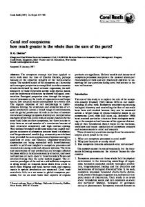
PC, and MLR. The error trends for Dataset 1 used in model calibration (figure 5), show that NSC has smaller errors than the other models in a large water depth range (from 2 to 17m). However, SC has a lower error than NSC at both extremes. In all water depths, PC, and MLR have higher errors than NSC. The error trend polynomial equation (figure 4(c)) shows that the NSC two-step procedure rms. has a quasi-linear relationship with depth. The computed bathymetry map using NSC is shown in figure 6.

5. Conclusions Water depth values were estimated in a coral reef area using four bathymetric models based on a T M image: PC,, MLR, NSC and SC. The rms. error for all the models increased as water depth increased, a trend that confirms the influence of water column attenuation on the model sensibility. In areas where changes in topography or bottom cover were highly variable, the rms. error was larger than in homogeneous areas (e.g. NSC rms. difference between datasets was 1.83 m). Among the models, PC, exhibited the largest rms. errors, suggesting that radiometric content not incorporated by PC, from original bands may influence bathymetiy estimations with emphasis in shallow areas. In contrast to the other models, SC had a different error pattern, exhibiting lower rms. errors in shallow and deep areas, with higher values close to 12m depth. The 3D scatterplot of DN values T M band 1, T M band 2 and T M band 3 from training areas showed a cluster of data points around a straight line for each water depth interval. These clusters gradually shifted from shallow to deep areas and produced an overlap among contiguous depth intervals. This overlap pattern could influence the rms. shape produced by SC. When total radiometric variability was reduced using NSC, and MLR was applied separately to

Assess~wr~t of coral reef bathjmetric mapping

-

O

m

m

h

(

D

"

7

(UJ)JOJJa

W

SWtl

n

N

-

Ail. A. Liceaga-Correa and J . I . Euan-Auila

Depth (m)

Figure 5. rms. error trend for each model from Dataset 1.

(Im 811m

1-2m

4 11-13m

2Jm

4 13-16m

4 34m 4 16-20m

4 44m >20m

4 5-7m 4 74m 4 Sand keys

Figure 6. Bathymetric map generated using non-supervised classification with multiple linear regression.

each region, a lower rms. error was obtained than whcn applying MLR to the whole image. Nonetheless, MLR showed results similar to NSC in waters from 6 to 12m depth. This cluster improvement clearly demonstrates that the NSC approach produces better estimations across the entire studied depth range. The water column characteristics and benthic patch distribution of reef habitats captured by the T M image were better incorporated in NSC. The low radiometric contributions of the water column due to the high transparency in the Alacranes Reef indicated that the influence of the bottom reflectance transmitted through the column is reduced when radiometric variability is segmented and treated separately. Acknowledgments This study was made possible by the Justo Sierra Regional Research System of the Consejo Nacional de Ciencia y Tecnologia (CONACyT). Travel facilities were provided by the Fleet Ministry of the Mexican Navy, and logistical support by the Sefialamiento Maritiino of the Secretaria de Comunicaciones y Transportes at Perez Island. We would also like to thank Dr Alfonso Condal for his useful comments, Htctor Rodriguez and Hector Hernandez for data and image processing, divers Javier Bello and Javier Axis, Guadalupe Mexicano for logistic assistance at CINVESTAV, and M r Luis Carlos Sosa Sanchez for safely navigating the maritime routes. Thanks are also due to reviewers for their useful comments and suggestions. References BADAN, S. M. J. B., 1993, The evaluation of different algorithms for bathymetric charting of lakes using Landsat imagery. I~~terrmtiond Journal of Reinote Sensirg, 14, 2263-2273.

BONET, F., 1967, Biogeologia subsuperficial del arrecife Alacranes, Yucatan. Boletin 80, Instituto de Geologia. Universidad Nacional Autonoma de Mexico.

C LARK . K. R.. T EMPLE. H. F., and C HARLES. L. W.. 1987, Bathymetry calculations with Landsat 4 TM imagery under a generalized ratio aswc~ption.Applied Optics, 26, 40364038.

C LARK , K. R.. T EMPLE H. F., and C HARLES L. W., 1988, Bathymetry using Thematic Mapper imagery. SPIE, 925, Ocecln Optics I X , 229-231.

GEORGE, D. G., 1997, Bathymetric mapping using a Compact Airborne Spectrographic Imager (CASI). Inter.ric~tiontrlJourncll of Remote Sensing, 18. 2067-2071.

G REEN , E. P., MUMDY, P. J., EDWARDS, A. J., and C LARK . C. D., 1996, A review of remote sensing for the assessment and management of tropical coastal resources. Cotrsml Mcl~~ogernent, 24, 1-40. HESSELMANS. G. H. F. M., WENSINK, G. J.: and C ALKOEN , C. J., 1994, The use of optical and SAR observations to assess bathymetric information in coastal areas. Proceedings of the in11 The~nclticConference 'Remote Sensing for Mevine Coasted En~ironrnents:New Orleclr~s,Vol. 1 (Ann Arbor, MI: ERIM), pp. 215-224. JOHNSON: R. W,, and MC'NDAY, J. C., Jr, 1983, The marine environment. In Mari~ledof Rrrnote Sensing, edited by R. M. Colwell, 2nd edn (Falls Church, Virginia: American Society of Photogrammetry), pp. 1440-1453. KHAN, M. A,, F ADLALLAH , Y. H.?and AL-HINAI, K. G., 1992, Thematic mapping of stibtidal coastal habitats in the western Arabia Gulf using Landsat T M data-Abu Ali Bay, Saudi Arabia. liiternational Jo~irnalof Remote Sensing, 13. 605-614. LILLESAND, T. M., and KIEFER, R. W., 1987, Remote Sensing and Inluge Interpretation, 2nd edn (New York: Wiley). L YZENGA, D. R., 1978, Passive remote sensing techniques for mapping water depth and bottom features. Applied Optics, 17, 379-383. LYZENGA, D. R., 1985, Shallow-water bathymetry using combined lidar and passive multispectral scanner data. Interncltionul Jo~irncdof Reinote Sensing, 6, 115-125. LUCZKOVICH, J. J., W A G N E R , T. W., M ICHALEK, J. L., and ATOFFLE, R. W., 1993, Discrimination of coral reef's, seagrass meadows. and sand bottom types from space: a Dominican Republic case study. Photogrnrnruetric Engineering and Rrrnote Sensing, 59, 385-389.

14

Assessn~entOJ'COI'LII r e e l batliyrnetric mupping

MARITORENA, S.. 1996, Remote sensing of the water attenuation in coral reefs: A case study Jollrnrrl of Remote Sensing, 17, 155-166. in French Polynesia. lnt~~rnatiorinl NEUMANN, G., and PIERSON. W. J. Jr, 1966, Principles of Phj~ricctlOceanograplr~~ (Englewood Cliffs, NJ: Prentice Hall). PIRAZZOLI, P. A,, 1985. Bathymetric mapping of coral reefs and atolls from satellite. Proceedirlgs of the Fifth lnronotiontrl C o r d Reef Congress. Tahiti, Vol. 6, pp. 539-544. P OLCYN, F. C., and SATTINCER, I. J., 1969, Water depth determination using renlote sensing techniques. Proceedings of the Sixth lnternnt~onalSynposii~rnon Rernote Sensing of the Enr~irornnent, held in Ann Arbor, hlichigcln, 13-16 October 1969 (Ann Arbor, MI: ERIM). pp. 1017-1028. SCHOWENCERDT, R. A,, 1997, Remote Sensing Models and Methodsfor ltnnge Processing, 2nd edn (San Diego, CA: Academic Press).