Assessment of Machining Models : Progress Report R.W. Ivester (2), M. Kennedy, M. Davies (1) National Institute of Standards and Technology1 Gaithersburg, MD 20899, USA Tel: 301/975-8324, Fax: 301/975-8058, e-mail:
[email protected] R. Stevenson, General Motors, Warren, MI, USA J. Thiele, Caterpillar Incorporated, Peoria, IL, USA R. Furness, S. Athavale, Ford Motor Company, Dearborn, MI, USA ABSTRACT Progress in developing and assessing predictive modeling of machining processes has been hindered by the extremely localized nonlinear physical phenomena that occur in machining and the many different types of models ranging from theoretical to empirical. The difficulty in assessing models has been cited by industry as the major barrier to use of modern machining models. Current practice in industry is to machine and change tools conservatively, or to conduct costly empirical studies for a limited selection of tools and coolants. The Assessment of Machining Models project will assess the ability of modern machining models to predict the outputs of machining processes based upon a consistent, well measured calibration data set. The data set is nearly complete and is to be used in benchmarking the predictive capability of machining models in blind tests. This paper presents the project motivation, goals, and representative calibration data set results. The next steps in the effort include release of the calibration data, solicitation and collection of predictions, and evaluation and reporting of results. MOTIVATION In 1998, Merchant estimated that 15 % of the value of all mechanical components manufactured worldwide is derived from machining operations [1]. Other studies have found that total U.S. expenditures on machining are between 3 % and 10 % of the annual U.S. gross domestic product (GDP): between $240 to $850 billion dollars for 1998 [2]. However, despite its obvious economic and technical importance, machining remains poorly understood. Parameters are chosen through empirical testing and the experience of machine operators and programmers. This 1
Official contribution of the National Institute of Standards and Technology; not subject to copyright in the United States.
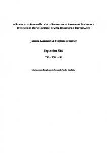
process is expensive and time-consuming. Furthermore, while large empirical databases have been compiled [3,4,5] to aid in process design, these databases lose relevance as new tool materials, machines, and workpiece materials are developed. For example, in the development of high-speed machining centers over the past ten years, speeds and feed rates have increased by an order of magnitude, rendering databases and handbook tables essentially useless. A number of recent industrial studies have illustrated the shortcomings in the current empirical methods of designing machining processes. For example, in an internal study, Kennametal gathered data over a one-year period (1992-1993) on the global use of cutting tools. This study found that in the United States: (1) the incorrect cutting tool is specified more than 50 % of the time; (2) tools are not used at the rated cutting speed in 42 % of applications; and (3) tools are not used to the end of life in 62 % of applications. An internal study at a major automotive manufacturer tracked the downtime on 111 different machine tools. The results of this study, partially detailed in Figure 1, indicate that 35 % of this downtime can be attributed to deficiencies in the performance of the machining process, with the remaining 38% and 27% attributed to blocking/starving and other causes, respectively. If these studies are truly representative of machining production in the United States the financial impact of the use of sub-optimal tooling selection, process parameters, and tool-change policies is staggering. An alternative approach to empirical testing and experience is the development of predictive models that are based upon the fundamental physics of the machining process. The advantage of this approach is that predictions are made from the basic physical properties of the tool and workpiece materials together with the kinematics and dynamics of the process. Thus, after the appropriate physical data is determined, the effect of changes in cutting conditions (e.g., tool geometry, cutting parameters, etc.) on industrially relevant decision criteria (e.g., wear rate, geometric conformance, surface quality, etc.) can be predicted without the need for new experiments. If robust predictive models can be developed, this approach would substantially reduce the cost of gathering empirical data and would provide a platform for a priori optimization of machining process parameters based upon the physics of the system. The difficulties in realizing true predictive models for machining arise from the extreme physical phenomena inherent in the system. Machining generates a highly inhomogeneous plastic flow where local stresses generate high rates of plastic deformation (up to 106 s-1) that give rise to inhomogeneous thermal fields, high temperatures (1200 ºC in machining steel), and high pressures (10 MPa). This type of complex plastic flow is difficult to predict even with sophisticated numerical software, and the basic data on material behavior under such conditions is nonexistent for most materials of practical interest [6,7]. These difficulties have forced model development to rely on various levels of empirical input data taken from machining tests (Figure 2) in order to model process variables of industrial
interest. The limitations imposed on the applicability of machining models by their reliance on empirical input data has limited their industrial use, particularly in smaller operations which are unable or unwilling to perform extensive validation testing. The goal of the Assessment of Machining Models effort is to provide an unbiased and anonymous assessment of the ability of current machining models to predict the practical behavior of machining processes. We make no attempt to restrict the definition of a model, other than to state that the models should be clearly defined in terms of the input data needed to make a prediction. For the purposes of the effort, we define a correct prediction as one that agrees with an experimental result to within a well-quantified experimental uncertainty. Thus to define an accurate prediction, the uncertainty inherent in machining systems must first be assessed by conducting experiments at multiple labs on different machines. The intent of the effort is to generate an experimental data set encompassing the inherent uncertainties associated with multiple laboratories and machining centers, provide an unbiased report of current capabilities for predicting the practical behavior of machining operations, and develop a roadmap for future directions in machining modeling research. BACKGROUND Machining research is driven by both ardent scientific curiosity and tremendous practical and financial utility. This dichotomy of motivations pervades the published literature. However, even though these two motivations are often at odds, neither can truly advance without the other. Without the practical utility, scientific studies are simply curiosities, and yet without a systematic scientific approach, the repeatability and overall utility of empirical machining studies is severely limited. The research literature on machining problems is vast (see for example Komanduri [8], Shaw [6]). Probably the earliest scientific report on the formation of a chip was presented in 1881 by A. Mallock [9] in the Proceedings of the Royal Society of London. Nearly coincident with the publication of Mallock’s article, F. W. Taylor was appointed foreman of the machine shop at the Midvale Steel Company, and over the next 25 years produced his now famous study of machining [3]. Thus, before the beginning of the 20th century, notable empirical and theoretical studies of machining were already underway. The next period of development occurred in the 1930’s and 1940’s. The study of machining mechanics was for the first time placed on a solid physical and mathematical foundation by the work of Piispanen [10], Ernst [11], and Merchant [12-15]. Since then, four formal categories of cutting models have emerged: (1) analytic models; (2) slip-line models; (3) mechanistic models; and (4) finite element models. Each approach has certain advantages and shortcomings. The choice of a particular cutting model depends on the information desired, the required accuracy
of this information, and the available resources. Availability of laboratory equipment enabling accurate process measurements is of paramount importance to the development of accurate models. The literature on experimental measurements in machining is extremely vast and therefore even a description of the most important results is beyond the scope of this paper. However, comprehensive review articles and textbooks can be consulted for further information and references [6,7,8]. Analytic models [16-22] establish relations between force components (e.g., between cutting and thrust forces and normal and tangential forces) based on the cutting geometry. These models are easy to use, but require prior knowledge of the shear angle, mean-friction angle, and chip-flow angle. These quantities must be determined experimentally, which limits the applicability and the accuracy of these models. Slip-line models [23-33] depend solely on material properties, rather than on experimental data. These models predict mechanical response and temperature distributions and are compatible with strain, strain-rate, and temperature-dependent models. However, the geometry of the slip-line field in the shear zone must be modeled, assumed, or somehow determined. Mechanistic modeling is a semi-empirical method capable of accurate prediction of cutting forces in a wide range of complex machining operations [34-47]. This approach is based on the assumption that cutting forces are proportional to the uncut chip area. The constant of proportionality, called the specific cutting energy, depends on the workpiece material, the cutting conditions, and the cutting geometry. The form of the function relating the specific cutting energy to the cutting geometry and conditions is assumed. The actual function is then determined by fitting experimental data in a process called calibration. Calibration can be based on simple orthogonal or oblique machining set-ups; geometric transformations can then be applied to predict cutting forces for a complex, three-dimensional machining process [43]. This simplifies the calibration set-up, but the need for testing is not eliminated and other important quantities such as tool chip interface temperatures are not predicted. Finite element models for machining processes were introduced in the early seventies [48,49]. Stevenson et al. conducted pioneering work in thermal finite element analysis of machining [50,51]. Lajczok [52] proposed a cutting model based on plane strain assumptions. Natarajan and Jeelani used a viscoplastic model to predict chip geometry [53]. Usui et. al. employed an incremental, elastic-plastic finite element model, starting from a steady-state solution [54,55]. Strenkowski and Carroll [56,57,58] also did pioneering work in finite element simulation of machining processes. More recently Marusich et al. [59] and Ceretti et al. [60,61,62] have developed more sophisticated schemes with adaptive remeshing that are capable of predicting non-steady chip formation. Today, the use of numerical cutting models is no longer limited to research; industry is starting to
adapt these methods to practical design applications. For example, Wayne et. al. make use of a commercial finite element code to predict chip flow [63]. Currently a major limit to the use of finite element software is the lack of fundamental materials data relevant to the conditions that occur in machining [64]. There are two main approaches to formulating finite element models for machining, Lagrangian models and Eulerian models. Lagrangian models track a fixed body of material as it approaches and passes the tool, while Eulerian models trace the flow of material through a fixed spatial domain in the vicinity of the tool. Lagrangian methods are well suited to simulating the entry and exit phases of chip formation as well as intermittent and discontinuous machining processes. They are compatible with elastoplastic material models [65,66]. On the other hand, Lagrangian models suffer a number of disadvantages. The large plastic deformations that occur in machining can generate unacceptable mesh distortion. It is difficult to construct a Lagrangian model for continuous tool advance through the workpiece; node-splitting methods [56-58,63,66] or continual remeshing [65, 59,60,62] are required to address this problem. Artificial parting criteria are required in node-splitting methods to determine when to advance the tool through the material [56-58,63,66]. It is also difficult to maintain grid alignment across slip interfaces, a problem that can lead to errors in predictions of thermal response. Lagrangian models are incompatible with direct steady-state solutions and relatively small time steps are required in transient solutions to capture the rapid changes that occur in the vicinity of the cutting tool. These features make Lagrangian finite element models computationally expensive. Eulerian models avoid problems of mesh distortion, since the mesh is constructed on a fixed domain. Relative material motion across a contact interface can be accommodated without sacrificing mesh compatibility [56-58,67-75]. Eulerian models capture the continuous flow of material around the tool, enabling a physically realistic model of machining of ductile materials, without remeshing or node-splitting. Direct steady-state solutions can be computed with Eulerian models, so they are computationally far less expensive than Lagrangian models for this class of problems. In transient problems, the solution at a fixed point in an Eulerian frame evolves more gradually than the solution at a fixed particle in a Lagrangian model. Therefore, larger time steps can be used without loss of accuracy in transient Eulerian models. On the other hand, Eulerian models require custom software development and are less well suited to modeling intermittent machining, entry and exit phases, and discontinuous chip formation (combined EulerianLagrangian (ALE) approaches [76, 77] might address these problems). The range and complexity of machining models across these four formal categories of analytic, slip-line, mechanistic and numerical models makes it extremely difficult to compare their utility and robustness. The quality of the output of models is uncertain, and there are no universal definitions of model inputs and outputs (e.g., some models may predict specific cutting energy from basic materials
properties while other models use specific cutting energy to predict the forces on a tool with complex shape). Unfortunately, these complexities and uncertainties often represent an unacceptable risk for the potential end-users of such models, who currently resort to heavily empirical (and costly) but reliable models such as Taylor tool-life curves. OBJECTIVES In an attempt to focus and better define the current state of machining research the following question was raised at the 1st International CIRP Workshop on Modeling of Machining Operations: “After 100 years of research in machining, why does industry still rely on 100 year old models to make predictions of what will be seen on the shop floor?” - Rich Furness, Ford Motor Company. The Assessment of Machining Models (AMM) effort arose from discussions motivated by this question. The goal of the project is to assess the ability of stateof-the-art machining models to make accurate predictions of the behavior of practical machining operations based upon the knowledge of machining parameters typically available on a modern industrial shop floor. It is important to note that from the industrial point-of-view, approximate predictions that can be made from machining parameters typically available on the shop floor would be more useful than more precise predictions based on less readily available model parameters. Critical assessment of model performance and robustness is necessary before such models can see widespread industrial use. In addition to assessing current prediction capabilities, the Assessment of Machining Models effort will assist in evaluating how close the modeling community is to the goal of practical predictive modeling of machining and where future research efforts in this area should be focused. In designing the effort it was asserted that any meaningful evaluation of model performance must have two characteristics. First, it must be based upon an accurate assessment of the uncertainty inherent in machining operations. Second, predictions must be conducted blindly (i.e., the predictor must have no a priori knowledge of the test results). To achieve the goal of the project, the following plan was developed by the project participants: 1. Provide a clear, consistent, well-measured, and relevant data set consisting of two components: a calibration data set that is fully disclosed; and a validation data set that is not disclosed until predictions have been submitted. Assess the uncertainties in the measurements. 2. Release the calibration data set and the parameters for the validation data set. 3. Solicit and collect voluntary blind predictions of the validation data set.
4. Provide an unbiased and anonymous reporting of the results. Organize a workshop to present and discuss the results of the project, and develop a roadmap for future research in predictive modeling of machining. These steps are discussed in more detail below. Data Generation: All data will be generated concurrently at the four different labs (NIST, Ford Motor Company, General Motors, and Caterpillar) and carefully compared prior to the solicitation of predictions. Lab-to-lab consistency provides a filter for identifying and correcting inconsistent or spurious experimental data and thereby ensuring that the data is accurate. In addition, the mean and standard deviation of the data will be calculated and used to define an accurate model, i.e., a model is considered accurate if it can consistently predict the standard deviations and the means of the validation data set. Data Release: Once consistent calibration and validation data sets are obtained, the calibration data set and the parameters for the validation data set will be publicly released via web site presentation, Internet downloads, and data storage media (Zip2 Disks, CD’s etc.). Solicitation and Collection of Blind Predictions: Solicitations for predictions will be sent to all parties who have expressed interest, and a general solicitation will be posted on the web. Predictions will be submitted on a voluntary basis. The due date for submission of predictions will be six months following the release of the data. Reporting of Results: An unbiased report of the results will be developed based on comparison of the predictions and the experimental data. This report will provide the focus for a workshop aimed at developing a roadmap for future work in the modeling of machining operations. The full calibration and validation data sets will be made available over the Internet for use in future modeling efforts. Currently, we are nearing the end of the data generation phase of the work. Approximately 30 international research groups have already expressed interest in participating in this study based upon responses to presentations of the planned activities at the International Mechanical Engineering Congress and Exhibition (IMECE) 1998 in Anaheim, the second CIRP modeling meeting in Nantes, France, January 1999, the North American Manufacturing Research Conference (NAMRC) 1999 in Berkeley, California, and IMECE 1999 in Nashville, Tennessee. Release of the data is scheduled for the end of the summer, 2000. During and after each of these presentations, the plan was strengthened in response to the comments and questions that arose. The remainder of the paper describes the design of the
2
Identification of specific commercial products is included in order to provide a complete description of the experimental work and does not imply endorsement by the National Institute of Standards and Technology, nor does it imply that the commercial products identified are necessarily the best for the purpose.
experiments for the effort and presents some representative samples of the experimental results. DESIGN OF THE EXPERIMENTS As stated above, the first step of the plan is to develop an accurate data set relevant to a common machining process used in industry. The choice of the process was primarily based upon input from the three industrial participants in the effort. All experiments will be done without coolant and will be repeated twice at each lab in order to obtain a statistical sampling of behavior. Choice of Process The process chosen was turning of American Iron and Steel Institute (AISI) 1045 steel using a general purpose tungsten carbide / cobalt (WC/Co) unalloyed carbide grade insert. The chemically simplest grade of carbide was chosen to simplify modeling tool-material behavior based on the material chemistry. Both uncoated and titanium nitride (TiN) coated inserts are used. The merits of this process are: (1) the machining of AISI 1045 steel has significant relevance in the automotive and heavy equipment industries; (2) the material properties of AISI 1045 steel and general grade carbide are well known; and (3) the workpiece and tool materials are easily obtainable in the configurations necessary for the tests. Test Configuration and Conditions Three types of experiments are being performed: (1) orthogonal machining using coated and uncoated inserts to generate a “calibration” data set; (2) orthogonal machining using machining parameters that fall both between and outside the parameters chosen for the calibration data set as part one of a validation data set; and (3) turning tests with uncoated inserts and with coated grooved (chip-breaker) inserts as part two of a validation data set. These experiments were chosen first to provide data to calibrate any models as necessary and second to provide a validation data set that tests model capabilities against problems of increasing difficulty. Given the current understanding of the physics of machining, it is likely that prediction of changes from orthogonal to non-orthogonal or non-orthogonal with a grooved insert is possible. However, because of changes in the tool-chip interface conditions, even if the properties of the coating are available, extrapolation from uncoated to coated conditions is much more difficult. The coated chip breaker cutting tests are most difficult of all to predict, yet they reflect current industrial practice. Workpiece Material and Geometry The workpiece material was AISI 1045 steel bar obtained from a single batch/heat. The material was machined to produce bars and tubes at NIST (National
Institute of Standards and Technology) and then distributed to the industrial laboratories. The dimensions of test workpieces were: Tubes - 152.4 mm overhang, 101.6 mm diameter, 1.6 mm wall thickness Bars - 101.6 mm overhang, 101.6 mm diameter. The material was subjected to chemical, mechanical, and metallurgical analysis as detailed in the next section. Tools and Toolholders Kennametal CTAPR 123 B toolholders were chosen for the experiments. These toolholders have three major advantages: (1) they are commercially available and so allow others to easily repeat the experiments in the future; (2) they have a simple geometric configuration with a 5º rake angle and a 0º included angle; and (3) they could be used for each of the cutting configurations. The inserts used were Kennametal grade K68. These inserts have the advantages: (1) they are commercially available; (2) they consist of a very simple WC/Co material; and (3) they come in configurations compatible with the toolholder and suitable for the desired cutting conditions. Custom ground angle plates were manufactured to mate with the toolholder and distributed by Kennametal to establish the desired rake angles of +5º, 0º and -7º without changing the toolholder. Observations of the initial tool edge radii for each of the types of inserts provide insight into the effect of tool coating on edge radius. Tool replications produced using a dental replicant (Dentsply Hydrosil) were sliced and examined under an optical microscope. Pictures of the sliced tool replications will be made available as part of the data release. Machine type and characterization The experiments were carried out simultaneously in the four test laboratories using CNC turret lathes as detailed in Table 1. While the results of several internal round robin tests done at one of the participating laboratories indicate that consistent machining behavior can be obtained on different equipment, it has been reported elsewhere that variations in dynamic behavior of machine tools can affect results. Particularly, rates of tool wear have been reported to be affected by the dynamics of the structural loop even under stable (non-chattering) cutting conditions. Thus, the dynamics of each machine tool will be characterized by NIST (with the dynamometer in the structural loop) using tool-tip frequency response functions measured with a piezoelectric hammer, signal analyzer, and accelerometer. Calibration Data Set Parameters A total of 16 orthogonal cutting tests were done to generate the calibration data set. The parameter values for both the coated and uncoated tools are shown in
Table 2. Test 5 is an accelerated wear test in which tool wear was measured as described below. The wear test is intended to provide data that can be used by modelers to “calibrate” the parameters in diffusion wear models. The parameter values were chosen to span a range of behaviors. According to data in Trent [7], all of these conditions will be free of a built-up edge, which would lead to unpredictable behavior and be impractical. According to Trent [7], machining of a low carbon steel with uncoated carbide under most of these conditions will lead to slow steady crater growth. Only the conditions for test 8 in Table 2 are likely to lead to rapid crater growth. Validation Data Set Parameters The validation data set consist of two major portions, orthogonal cutting and turning tests. The orthogonal tests were conducted with the parameter values given in Table 3. These parameters will test both the interpolation and extrapolation capability of the models. The turning tests are also chosen to require interpolation and extrapolation of the orthogonal cutting data. The cutting conditions for these tests are summarized in Table 4. Each experiment will be conducted using uncoated flat-faced inserts and TiN coated grooved inserts. As mentioned above, this battery of experiments was chosen to provide a progressively increasing level of modeling difficulty. Measured Quantities Forces, temperatures and wear were measured using the methods detailed below for the conditions detailed in Tables 2-4. For all of the calibration tests in Table 2 except test 5 and all of the validation orthogonal tests (Table 3) no wear results were measured. Chip morphology measurements were made for the orthogonal cutting tests in the calibration data set. These include measurements of the chip thickness and width after machining. Because measurements of contact length can be ambiguous, contact length was not measured; however, it could be inferred for some of the tests from the wear patterns that occur (see Accelerated Wear Test section). Forces Forces were measured using Kistler 3-axis piezoelectric dynamometers as detailed in Table 1. The tools were mounted to the dynamometer using Kistler toolholder mounts as detailed in Table 1. The rake angles were established using custom ground angle brackets from Kennametal. An example of the dynamometer toolholder set-up is shown in Figure 3.
Temperatures Average temperatures were measured using two methods. All tests were measured using an intrinsic thermocouple at industrial lab 3 and NIST, and selected measurements are being made at NIST using IR microscopy. The intrinsic thermocouple uses the bi-conducting tool-chip interface as a thermocouple junction. First the toolholder was electrically isolated from the remainder of the machine using a Bakelite spacer between the dynamometer and the Kistler toolholder mount. Bakelite washers were also placed between the screw heads and the toolholder. One wire was then mounted to a slip ring on the back of the spindle and the other to the tool holder. The calibration procedure for the intrinsic thermocouples involves placing the Kennametal toolholder in contact with a workpiece and observing the output voltage while heating the toolholder and workpiece at the contact point and measuring the temperature with a conventional thermocouple. The intrinsic thermocouple systems have not yet been calibrated. As such, only comparisons of the voltages measured by NIST and industrial lab 3 can be made until the systems have been calibrated. While this method has been used for some time in experimental research [78,79,80,81] it does have the following documented shortcomings: (1) it reports some weighted integration of the temperatures across the tool-chip interface surface; (2) it is affected by other biconductor interfaces in the measurement loop; and (3) it is affected by (unknown) fluctuations in tool-chip contact area. However, this method remains one of the most robust and reliable methods for assessing changes in mean tool-chip interface temperatures. Therefore, it was chosen as the main method of temperature measurement for this effort. As part of a separate project at NIST a thermal imaging micro-pyrometer (MIPY) was constructed using a commercial 128 by 128 indium antimony (InSb) focal plane array (FPA) with an all-reflective 0.5 numerical aperture (NA) and 15x microscope objective that directly focused the image of the object on the FPA. The InSb detector was used with a broad-band spectral filter, which transmits from 3 µm to 5 µm in wavelength, and the spatial resolution of the system was estimated to be approximately equal to the wavelength of the detected light from using the Rayleigh criterion. The individual pixels in the FPA were deposited 50 µm apart resulting in a spatial resolution of at best < 5 µm per pixel, and the spatial resolution was further verified using a chrome-on-glass USAF 1951 resolution target. The system was calibrated using a NIST miniature blackbody with a 2 mm aperture. The emissivity of the steel was measured as a function of temperature using a reflectance technique. Due to the nonlinear calibration curve of the detector and the nonlinear temperature variation of the emmissivity, an iterative procedure was required to obtain material temperature from the measured signals. To reduce error motions and maintain focus the thermal microscopy system was mounted on a high-load capacity air-bearing spindle configured to conduct orthogonal cutting as shown in Figure 4a. This
system will be used to provide some limited thermal maps of machining AISI 1045 steel for the AMM project. Wear Wear measurements were conducted according to ISO 3685. The following methods of measuring wear patterns were investigated and compared: (1) air bearing linearly variable differential transducer (LVDT) (crater depth); (2) whitelight interferometer (500 micrometer vertical travel with 10 nm resolution and 5 mm by 5 mm field of view using a 2.5x objective); (3) replication techniques; (4) optical microscope; and (5) scanning electron microscope. The first three methods were used to quantitatively measure crater geometry. The optical microscope was used to measure crater depth and flank wear shape. The SEM was used primarily for qualitative imaging of worn tools. Chip Morphology For each of the tests the machined chips were collected and classified according to type as specified in ISO 3685 Table G1. For the orthogonal cutting tests, the thickness and width of the chips were measured after machining. By combining these measurements and the forces a table (see below) of relevant physical quantities (e.g., shear angle, shear and friction forces, etc.) was populated using the classical Merchant model. GENERATION OF THE CALIBRATION DATA SET This section details the generation of the calibration data set and provides some sample results that demonstrate the approach and the level of lab-to-lab consistency obtained. Material Characterization The material was ordered as a single batch of AISI 1045 steel, 30.5 m (100 ft) of 101.6 mm (4 in) diameter rod in 5 rods, each 6.1 m (20 ft) long. The 5 rods were cut into a combination of 152.4 mm (6 in) and 203.2 mm (8 in) long bars, with a 50.8 mm (2 in) thick circular sample removed from each end. The ten samples were subjected to chemical and metallurgical analysis using American Society for Testing and Materials (ASTM) test procedures E3-95, E407-93, E112-95, E1019-94, and E415-95a. Grain sizes were measured quantitatively using an optical microscope. Additionally, Brinell hardness measurements and a series of ultrasonic nondestructive evaluations were performed on a sampling of the bars. The chemical analysis results are shown in Table 5. The chemical content did not vary significantly among the ten samples as indicated by the average and standard deviation of the measurements given in Table 5. The material conforms to the military specification (milspec) for AISI 1045, and satisfies the more stringent
ISO C45 standard except for copper content, which is slightly high. The grain size ranges were measured for each sample. The lower and upper bounds of these ranges averaged 3.4 and 7.55, with standard deviations and repeatability uncertainties of 0.7 and 0.1, respectively, for both the upper and the lower bounds. The resulting ±2s expanded uncertainty [82] on the upper and lower bounds is ±0.71. Four representative pictures of longitudinal and transverse cross-sections from two of the samples are shown in Figure 5. Brinell Hardness measurements were performed on two of the 150-mm long workpiece bars with a 29.4 kN load and 10-mm ball. For each of the bars, six measurements were made on one face approximately 1 cm away from the center of the face in a circular pattern around the center. The diameters of the resulting impressions left on the bars were measured at 4.3 mm each with a measurement precision of ±0.025 mm. This equates to a Brinell Hardness Number (BHN) with a ±2s expanded uncertainty of 196 ±5 [81]. Ultrasonic examinations of the workpiece material were also performed on four of the 150-mm long bars before they were machined into tubes. Two different types of pulse-echo ultrasonic contact tests were performed with an orientation parallel to the axis of the cylinder. One using longitudinally oriented waves, and the other using transverse waves. The results of the two pulse-echo ultrasonic tests enable the speed of sound through the material to be estimated, and thus the consistency of the bulk elastic modulus and density can be characterized. On each of four bars, measurements of length were taken with a caliper, and elapsed time between ultrasonic pulses and echoes were recorded on an oscilloscope. The measured values of the speed of longitudinal and transverse ultrasonic waves in the bars were found to be in reasonable agreement with the handbook values [83] for steel, 5,900 m/s and 3,230 m/s respectively. Additionally, the transducer was moved continuously in circular rings around the center of the bars’ circular ends. No distinguishing features were observed among the four bars judging from the echo amplitude pattern. Had there been any large differences in the density or microstructure of the material a visible difference would have been observed in the echo pattern. The results of the chemical analysis, hardness tests, and ultrasonic examinations establish that the original material was mechanically and chemically suitable for use in the machining tests. Preparation of Workpieces The material arrived at NIST in 5 bars each approximately 6 m in length. The bars were rough-sawed into shorter bars 150 mm and 200 mm long for use in the orthogonal and turning tests, respectively. The short bars were then faced and numbered in the order they were cut from the long bars. Parts were stamped with a 3
digit number, with the first digit for the bar number out of the original 5 and the second and third digits for the part number within the bar (01-36). In order to address the possibility of variation among the tubes by location within the original bar, the bars were distributed to the four labs in a staggered order. The outer diameter of the 200 mm bars was finish turned to remove scale. The 150 mm bars were machined into tubes for orthogonal cutting through a series of operations including drilling, rough and finish boring of the internal diameter, and finish turning of the outer diameter. The cores of the 150 mm bars were drilled out to a depth of 100 mm on a manual lathe using a 31.75 mm (1.25 in) diameter 118° included angle tapered shank drill bit. The drilled hole was then rough bored at 245 rpm spindle speed, 22.4 mm/min feed rate, and 2.54 mm depth of cut. Finish boring was performed at 165 rpm spindle speed, 38.1 mm/min feed rate and 0.56 mm depth of cut. All boring was performed with a Carboloy S16SCLCL-3 boring bar and a SECO CCMT 32.52-F2 TP30 insert. Finish turning of the outer diameter was performed with a Kennametal CN42 80° Diamond K68 grade coated insert at 300 rpm spindle speed, 38.1 mm/min feed rate, and 0.89 mm depth of cut. The length of cut for all operations was 101.6 mm. Wall thickness measurements were performed to ensure consistency. The ±2s expanded uncertainty [81] for the 1.6 mm wall thickness was ±0.05 mm. Characterization of Experimental Apparatus The tool holder and mount and dynamometer were assembled as shown in Figure 3. The dynamic stiffness of both of the lathes to be used for the experiments at NIST was measured. The frequency response function (FRF) for the Hardinge Superslant is given in Figure 6. The ±2s expanded uncertainties for the peak/valley heights and frequencies are ±10 % and ±5 %, respectively. Forces While the raw data for the calibration cutting experiments will be released in its entirety, full presentation of the raw data would be impractical in this paper. Instead, representative samples of the wear progressions are given, and averages of the forces and intrinsic thermocouple voltages are given for the full data set. The average forces for the orthogonal cutting tests with coated and uncoated flat inserts for experiments conducted at all four laboratories are shown in Figure 7. In this graph, the cutting forces are negative and the thrust forces are positive, as produced by the Kistler Dynamometer in the cutting setup used. The lines represent ±2sI expanded uncertainty for the set of all force averages from the four labs for test condition i. The consistency between the four laboratories is sufficient to allow differences in forces due to parameter variations to be discerned.
Accelerated Wear Test Figure 8 shows two wear progressions for experiments conducted at NIST. Cutting was stopped every 5 mm of tube length and the insert was examined with an optical microscope, an LVDT air bearing indicator, and a white-light interferometer. Wear measurements were taken following procedures detailed in ISO 3685. The two wear progressions shown are for nominally identical cutting conditions and demonstrate a high degree of repeatability in the wear progression. The squares and diamonds represent LVDT measurements of peak crater depth. The triangles represent measurements of peak crater depth from the interferometer. The five interferograms used are shown inset on the figure adjacent to the corresponding data points. Chip Morphology For each of the calibration tests in Table 2, the final chip thickness and width was estimated based on the average of many individual measurements with a dial caliper, and the shear angle was calculated based upon the assumption that the Merchant model was valid. The shear angle, F , was calculated as F =atan[r*cos(a)/(1-r*sin(a))], where a is the rake angle, and r is the chip thickness ratio. It is important to note that the chip width varies considerably, which violates the assumptions for the Merchant model. The ±2s expanded uncertainty for NIST measurements is less than ±100 µm. The averages of chip measurements are given in Table 6. Representative Temperature Data The primary temperature measurement method was the intrinsic thermocouple. The signals measured through the coated inserts were not found to be sufficiently consistent to be a meaningful representation of the average temperature at the toolchip interface surface. Figure 9 shows the averages and ±2s expanded uncertainties of the intrinsic work-tool thermocouple voltage outputs for each of the calibration data set tests with uncoated inserts. The clearest trend in the changes of thermocouple voltage with test number are between test 1-2 and 3-4, where the rake angle changes from –7° to +5°, and between tests 1-4 and tests 5-8, where the changes between the ordered pairs from these sets (1 and 5, 2 and 6, etc.) are an increase in cutting speed from 200 m/min to 300 m/min. Figure 10 shows a representative thermal profile of machining with the cutting conditions indicated in the caption. While these conditions are not as aggressive as those used in the calibration data set, they do serve to demonstrate the resolution and capability of the system. The white lines on the figure represent the tool and workpiece surfaces in the plane. The peak temperature is approximately 650 °C and occurs at a point about 140 µm from the cutting edge of the tool. This is consistent with other findings as well as tool wear patterns and is a result of the highly
localized plastic flow that occurs at the boundary of the tool and chip. The ±2s expanded uncertainties in these measurements from all sources are less than ±30 °C. FUTURE WORK AND TIMETABLE Currently, the calibration data set is nearly complete. The future steps in the effort are described below. Release of Calibration Data The calibration data will be released during the summer of 2000. The primary method of release will be through downloads from the project’s web site, located at http://www.nist.gov/amm/. The web site is used for reporting progress, disseminating the model reference data and input parameters as described above, and collecting prediction reports. The calibration data set will be provided in a spreadsheet format that will include a template for submitting results. At the time of data release, all groups who have expressed an interest in submitting predictions will be contacted via email. Solicitation and Collection of Predictions All parties who have expressed interest in AMM at various workshops will be invited to provide predictions. After the release of the calibration data set, a sixmonth deadline for submission of predictions will be established. By that deadline all prediction reports will be electronically submitted to NIST via the project web site. Evaluation and Reporting of Results A committee of representatives from the four industrial participants will meet to discuss the results. At this meeting the results will be discussed and a final report will be generated. The report will objectively and impartially document the results and make suggestions for future work in the area of modeling of machining. Also at this time, a workshop at NIST will be held to discuss future work. All of the modeling participants will be invited to attend the workshop. Some of the modeling participants may be invited to make presentations at this workshop. SUMMARY The project plan and experimental procedure were designed to result in acceptable control of experimental consistency. Based on the results presented in this paper, the lab-to-lab consistency is acceptably good. This effort will result in an unbiased assessment of the current capabilities of machining models.
ACKNOWLEDGEMENTS We would like to take this opportunity to thank the many people who have contributed to the development and implementation of this effort, including Ranajit Ghosh, Ming Leu, Vivek Chandrasekharan, Bob Polvani, Tony Schmitz, Dieter Ebner, Wendy Shefelbine, and Gerry Blessing. This work was supported in part by National Science Foundation Grant Number 9909130. REFERENCES 1. Merchant, E., 1998, Proceedings of the CIRP International Workshop on Modeling of Machining Operations, Atlanta, GA, USA. 2. Soons, H.A., Yaniv, S.L., 1995, Precision in machining : research challenges, Gaithersburg, MD : National Institute of Standards and Technology, NISTIR 5628. 3. Taylor, F. W., 1907, Trans. ASME 28:31. 4. Koenigsburger, F., 1964, Design Principals of Metal Cutting Machine Tools, Peragamon, Oxford. 5. Machining Data Handbook, 3rd Edition, 1980, Vol. 1 & 2, Metcut Reseach Associates Inc., Cinncinnatti, Ohio, USA. 6. Shaw, M. C., 1984, Metal Cutting Principals, Oxford Press, Oxford, UK. 7. Trent, 1991, Metal Cutting, Butterworth-Heinemann, Oxford. 8. Komanduri, R., 1993, Appl Mech Rev, 46(3), 80-129. 9. Mallock, A., 1881, Proc. Royal Soc (Lon), 33:127-139. 10. Piispanen, V., 1937, Teknillan Aiakakauslenti 27:315. 11. Ernst, H., 1938, Physics of Metal Cutting, Machining of Metals, ASM, 1-34. 12. Ernst, H., Merchant, M. E., 1941, Trans. ASME 29:299. 13. Merchant, M. E., 1945, Trans. ASME, 66:A65-A71. 14. Merchant, M. E., 1945, J. App. Phys.,16:267. 15. Merchant, M. E., 1945, J. App. Phys., 16:318. 16. Ernst, H., Merchant, M.E., 1941, Chip formation, friction and high quality machined surfaces, Surface Treatment of Metals, Vol. 29, p. 299. 17. Merchant, M.E., 1945, Mechanics of the cutting process, Journal of Applied Physics, Vol. 16, p. 267 -318. 18. Lee, E.H., Schaffer, B.W., 1951, The theory of plasticity applied to a problem of machining, Journal of Applied Mechanics, Vol. 18(4), p. 405. 19. Rubenstein, C. ,1983, The mechanics of continuous chip formation in oblique cutting in the absence of chip distortion, part 1 – theory, International Journal of Machine Tool Design and Research, Vol. 23, No.1, pp. 11-20.
20. Lau, W. S., Rubenstein, C., 1983, The mechanics of continuous chip formation in oblique cutting in the absence of chip distortion, part 2 - comparison of experimental data with the deductions from theory, International Journal of Machine Tool Design and Research, Vol. 23, No.1, pp. 21 -37. 21. Grzesik, W., 1990, The mechanics of continuous chip formation in oblique cutting with single-edged tool - part I. theory, International Journal of Machine Tool Manufacturing, Vol. 30, No. 3, pp. 359-371. 22. Grzesik, W., 1990, The mechanics of continuous chip formation in obliquecutting with single-edged tool - part II. experimental verification of the theory, International Journal of Machine Tool Manufacturing, Vol. 30, No. 3, pp. 373-388. 23. Palmer, W.B., Oxley, P.L.B., 1959, Mechanics of metal cutting, Proceedings of Institute of Mechanical Engineers, Vol. 173, p. 623. 24. Oxley, P.L.B., 1961, A strain hardening solution for the shear angle in orthogonal metal cutting, International Journal of Mechanical Sciences, Vol. 3, p. 68. 25. Johnson, W., 1962, Some slip-line fields for swaging or expanding, indenting, extruding and machining with curved dies, International Journal of Mechanical Sciences, Vol. 4, p. 323. 26. Oxley, P.L.B., Hatton, A.P., 1963, Shear angle solution based on experimental shear zone and tool-chip interface stress distribution,International Journal of Mechanical Sciences, Vol. 5, p. 41. 27. Oxley, P.L.B., Welsh, M.J.M., 1963, Calculating the shear angle in orthogonal metal cutting from fundamental stress, strain, strain-rate properties of the work material, Proceedings 4th International Machine Tool Design and Research Conference. Pergamon, Oxford, p. 73. 28. Usui, E., Hoshi, K., 1963, Slip-line fields in metal cutting involving centered fan fields, International Research in Production Engineering ASME, p. 61. 29. Kudo, H., 1965, Some new slip-line solutions for two-dimensional steady-state machining, International Journal of Mechanical Sciences, Vol. 7, p. 43. 30. Fenton, R.G., Oxley, P.L.B., 1968, Mechanics of orthogonal machining : allowing for the effects of strain-rate and temperature on tool-chip friction, Proceedings of Institute of Mechanical Engineering. 31. Dewhurst, P., Collins, I.F., 1973, A matrix technique for constructing slip-line field solutions to a class of plane-strain plasticity problems, International Journal of Numerical Methods in Engineering, Vol. 7, p. 357. 32. Dewhurst, P., 1978, On the non-uniqueness of the machining process, Proceedings of Royal Society, London, Vol. A360, p. 587. 33. Dewhurst, P., 1979, The effect of chip breaker constraints on mechanics of machining, Annals of CIRP, Vol. 28, p. 1-5.
34. Martelloti, M.E., 1941, An analysis of the milling process, Trans. ASME, Vol. 63, p. 667. 35. Martelloti, M.E., 1945, An analysis of the milling process II : down milling, Trans. ASME, Vol. 67, p. 233. 36. Koenigsberger, F., Sabberwal, A.J.P.,1960, Chip section and cutting force during the milling operation, Anals of CIRP. 37. Kline, W.A., DeVor, R.E., 1983, The effect of runout on cutting geometry and forces in end milling, International Journal of Machine Tool Design and Research, Vol 23, No. 2/3, p. 123-140. 38. Nakayama, K., Arai, M., Takei, K., 1983, Semi-empirical equations for three components of resultant cutting force, Anals of CIRP, Vol. 30, No. 1, p. 33. 39. Fu, H.J., DeVor, R.E., Kapoor, S.G., 1984, A mechanistic model for the prediction of the force system in face milling operations, ASME Journal of Engineering for Industry, Vol. 106, p. 81-88. 40. Subramani, G.R., Suvada, R., Kapoor, S.G., DeVor, R.E., Meingast, W., 1987, A model for the prediction of force system for cylinder boring process, Proc. NAMRC 15, pp. 439-446. 41. Smith, S. and Tlusty, J., 1988, Modeling and the simulation of the milling process, ASME, PED-Vol. 33, Proc. Winter Annual Meeting, pp. 17-26. 42. Chandrasekharan, V., Kapoor, S.G., DeVor, R.E., 1993, A mechanistic approach to predicting the cutting forces in drilling : with application to fiberreinforced composite materials, ASME, MD-Vol. 45/PED-Vol. 66, Proc. Machining of Advanced Composites, pp. 33 - 51. 43. Endres, W.J., DeVor, R.E., Kapoor, S.G., 1993, A dual-mechanism approach to the prediction of machining forces, Parts 1 and 2, Proc., ASME Sym. on Modeling, Monitoring and Control Issues in Manufac., PED-Vol. 64, pp. 563593. 44. Jawahir, I. S., 1986, Ph.D. Thesis, University of New South Whales. 45. Amarego, E.J.A., Brown, R.H., 1969, The Machining of Metals, Prentice Hall, Engelwood Cliffs New Jersey. 46. Budak, E., Altintas, Y., Amarego, E.J.A., 1996, J. Man. Sci. Eng., 118: 216-224. 47. Amarego, E.J.A., Uthaichaya, M., Journal of Engineering Production 1(1):1-18. 48. Okushima, K., Kakino, Y., 1971, The residual stress produced by metal cutting, Annals of CIRP, Vol. 20(1), p. 13. 49. Klamecki, B.E., 1973, Incipient chip formation in metal cutting - a three dimension finite element analysis, Ph.D. Dissertation, University of Illinois at Urbana-Champaign.
50. Tay, A.O., Stevenson, M.G., Davis, G.D.V., 1974, Using finite element method to determine the temperature distribution in orthogonal machining, Proceedings of Institute of Mechanical Engineers, Vol. 188, p. 627. 51. Stevenson, M.G., Wright, P.K., Chow, J.G., 1983, Further developments in applying finite element technique to the calculation of temperature distributions in machining and comparisons with experiment," Journal of Industry, Vol. 105, p. 149. 52. Lajczok, M.R., 1980, A study of some aspects of metal machining using finite element method, PhD Dissertation, North Carolina State University. 53. Natarajan, R., Jeelani, S., 1983, Residual stresses in machining using finite element method, Computers in Engineering, Computer Software and Applications, Vol. 3, p. 79. 54. Shirakashi, T., Usui, E., 1974, Simulation of orthogonal cutting mechanism, Proceedings of International Conference of Production Engineering, Tokyo, p. 535. 55. Usui, E., Shirakashi, T., 1982, Mechanics of machining from descriptive to predictive theory, On the Art of Cutting Metals - 75 Years Later, ASME Publication PED, Vol. 7, p. 13. 56. Strenkowski, J.S., Carroll III, J.T., 1986, An orthogonal metal cutting model based on an Eulerian finite element method, Manufacturing Processes, Machines and Systems, Proceedings of the 13th NSF Conference on Production Research and Technology. 57. Carroll III, J. T., 1986, A numerical and experimental study of single point diamond machining, PhD Thesis, North Carolina State University. 58. Carroll III, J.T., Strenkowski, J.S., 1988, Finite Element Models of Orthogonal Cutting with Application to Single Point Diamond Turning, International Journal of Mechanical Sciences, Vol. 30, p. 899-920. 59. Marusich, T. D., Ortiz, M., 1995, Int J. Numer. Methods Eng. 38:3675. 60. Ceretti, E., Fallbohmer, P., Wu, W.T., Altan, T., Int. J. Mat. Proc. Tech., 59:169. 61. Maekawa, K., 1999, Application of 3D Machining Modeling to Cutting Tool Design, Proceedings of the IInd CIRP Int’l Workshop on Modeling of Machining Operations, Nantes, France. 62. Ceretti, E., 1999, Numerical Study of Segmented Chop Formation in Orthogonal Cutting, Proceedings of the IInd CIRP Int’l Workshop on Modeling of Machining Operations, Nantes, France. 63. Wayne, S.F., Zimmerman, C., O’Niel, D.A., 1993, Aspects of advanced cutting tool and chip-flow modeling, Proceedings of the 13th International Plansee Seminar, Eds. H. Bildstein and R. Eck, Metallwerk Plansee, Reutte Vol. 2, p.64.
64. Childs, T., 1997, Material Property requirements for modeling metal machining, J. Phys. IV France 7 Colloque C3, suppl. Au J. Phys. III. 65. Camacho, G., Marusich, T., Ortiz, M., 1993, Adaptive meshing methods for the analysis of unconstrained plastic flow, Advanced Computational Methods for Material Modeling, Eds. Benson, D. J. and Asaro, R. J., ASME AMD-Vol. 180/PVP-Vol.268, pp. 71 - 83. 66. Lin, Z.C., Chu, K.T., Pan, W.C., 1994, A study of the stress, strain and temperature distributions of a machined workpiece using a thermo-elastic-plastic coupled model, Journal of Materials Processing Technology, Vol. 41, pp. 291310. 67. Strenkowski, J.S., Moon, K.J., 1990, Finite Element Prediction of Chip Geometry and Tool/Workpiece Temperature Distributions in Orthogonal Cutting, ASME Journal of Engineering for Industry, Vol. 112, p. 313-318. 68. Moon, K.J., 1988, A thermo-viscoplastic model of orthogonal cutting including chip geometry and temperature prediction, Ph.D. Thesis, North Carolina State University. 69. Strenkowski, J.S., Moon, K.J., 1989, A thermo-viscoplastic model of the cutting process including chip geometry and temperature prediction, Advances in Manufacturing Systems Integration and Processes, 15th Conference on Production Research and Technology. 70. Hsu, J.M., 1990, Three-dimensional finite element modeling of metal cutting, Ph.D. Thesis, North Carolina State University. 71. Chern, S.Y., 1991, An improved finite element model of orthogonal cutting with special emphasis on a separate shear zone model, Ph.D. Thesis, North Carolina State University. 72. Hsu, H.C., 1992, An elasto-viscoplastic finite element model of orthogonal metal cutting for residual stress prediction, Ph.D. Thesis, North Carolina State University. 73. Chien, W.T., 1992, A numerical and experimental investigation of the sticking and sliding contact regions at the chip-tool interface in machining Aluminum 6061-T6, Ph.D. Thesis, North Carolina State University. 74. Yang, J.A., 1992, A predictive model of chip breaking for groove-type tools in orthogonal machining of AISI 1020 steel, Ph.D. Thesis, North Carolina State University. 75. Athavale, S.M., 1994, A damage-based model for predicting chip breakability for obstruction and groove tools, Ph.D. Thesis, North Carolina State University. 76. Liu, W.K., Chang, H., Chen, J.S., Belytschko, 1988, "Arbitrary LagrangianEulerian Petrov-Galerkin Finite Elements for Nonlinear Continua," Computer Methods in Applied Mechanics and Engineering, Vol. 68, pp. 259-310.
77. Movahhedy, M., Gadala, M.S., Altintas, Y., 2000, "Simulation of the Orthogonal Metal Cutting Process using an Arbitrary Lagrangian-Eulerian Finite Elemend Method," J. of Materials Processing Technology, Vol. 103, pp.267275. 78. Herbert, E.G., 1926, The Measurement of Cutting Temperatures, Proceedings of the Institute of Mechanical Engineers, pp. 289-329. 79. Boston, O.W., Gilbert, W.W., 1935, Cutting Temperatures Developed by Single-Point Turning Tools, Trans. of the ASM, vol. 23, pp. 703-726. 80. Trigger, K.J., 1948, Progress Report No. 1 on Tool-Chip Interface Temperatures, Transactions of the ASME, Vol. 70, pp. 91-98. 81. Stephenson, D.A., 1993, Tool-Work Thermocouple Temperature Measurements – Theory and Implementation Issues, ASME Journal of Engineering for Industry, Vol. 115, pp. 432-437. 82. Taylor, B.N., and Kuyatt, C.E., 1994, Guidelines for Evaluating and Expressing the Uncertainty of NIST Measurement Results, National Institute of Standards and Technology Technical Note (TN) 1297. 83. Nondestructive Testing Handbook, 1991, 2nd Edition, Volume 7, Ultrasonic Testing, American Society for Nondestructive Testing.
Lubrication 27% Other Downtime
Coolant 3% 2% 2%
Setup/Changeovers 9% 1% Start Up Speed10%
8% Fixtures
Blocked/Starved 38%
Tooling related Figure 1: Downtime on 111 machine tools at a major U.S. automotive company
3D, Empirical, Mechanistic 3D, Analytic 2D, FEM 2D, Thick Zone, Slip-line 2D, Thin Zone, Analytic 1937
1947
1957
1967
1977
1987
Figure 2: Timeline showing the history of the development of models.
1997
Figure 3 : Photograph of the tool, dynamometer, and the intrinsic thermocouple.
1 4 5
2
3
( a) V
Chip
Tool
Ω
Shear Zone Feed ( f) (b)
Figure 4: (a) Photograph of the experimental system showing: (1) air bearing spindle; (2) AISI 1045 steel tube; (3) monolithic tool post; (4) zero rake angle tungsten carbide insert; (5) micropyrometry system. (b) Schematic diagram of orthogonal cutting, a cutting configuration that generates a nearly two-dimensional plastic flow of material.
Figure 5 : Micrographs of polished and etched longitudinal and transverse sections of bar caps
Frequency Response Function for Lathe at NIST 0.0000003
0.0000002
Real (m/N)
0.0000001
0
-0.0000001
-0.0000002
-0.0000003 1.00E-06
100
200
300
400
500
Frequency (Hz)
Frequency Response Function for Lathe at NIST 0
-0.0000001
Imaginary (m/N)
-0.0000002
-0.0000003
-0.0000004
-0.0000005
-0.0000006
-0.0000007 1.00E-06
100
200
300
400
500
Frequency (Hz)
Figure 6 : Real and imaginary components of the frequency response measured at the tool tip on the NIST Hardinge lathe. The x- y- and z-omponents are shown in solid, dashed, and dash-dotted lines, respectively. The ±2s expanded uncertainties on the peak/valley heights and frequencies are ±10 % and ±5 %, respectively.
AMM Cutting Data NIST, Cat, GM Tangential (Cutting) Forces, Uncoated Inserts 1000 800 600
Cutting Force (N)
400 200 0 -200 -400 -600 -800 -1000 -1200 -1400 1 2 3 4 5 6 7 8 9 10 11 12 13 14 15 16 Test Number Figure 7 : Force data for the calibration tests from all four labs. NIST data is shown as diamonds, industrial labs 1, 2, and 3 are shown as squares, circles, and crosses, respectively. The lines bounding the data points represent ±2s expanded uncertainty on the data points for all four labs. The upper trace is thrust force, the middle trace is the out of plane force, and the lower (negative) force is the cutting force.
140
Crater Depth (um)
120 100 80 60 40 20 0 0
20
40
60
80
100
120
140
160
Length of Cut (m )
Figure 8: Measured tool wear progression in two orthogonal wear tests showing white light interferometer measurements (triangles and overlays) and LVDT measurements (squares and diamonds). Overlays are three-dimensional crater depth plots, with the cutting edge at the top. The depth scale for these overlays is shown on the right. Expanded uncertainties (±2s) on LVDT measurements and interferometer measurements are ±5µm.
Thermocouple Voltage vs. Test Number
Thermocouple Voltage (V)
0.016 0.014 0.012 0.01 0.008 0.006 0.004 0.002 0 1
2
3
4
5
6
7
8
Test Number
Figure 9: Average thermocouple voltages for uncoated calibration tests. Diamonds and crosses represent measurements performed at NIST and industrial lab 3, respectively. Dashes represent ±2s expanded uncertainties on data points from both labs.
Tool
Y (µm)
T (°C)
Workpiece
X (µm)
Figure 10: Temperature map of orthogonal cutting with a zero-rake cutting tool using a cutting speed of 3.7 m/s, and an uncut chip thickness of 50 micrometers.
Lab Industrial Lab 1 Industrial Lab 2
Machine OKUMA CadetL1420 X650 CNC (3500 rpm, 22 kW) Lelond Makino Baron 60 Lathe (37 kW) Okuma LC-20 Lathe (3000 rpm, 15 kW)
Force Kistler
Tool Wear Wild Heerbrug MPS 11 Optical Microscope Optical Microscope
Kistler 9257B and 9403 mount Industrial Kistler 9257 B Wyko white-light Lab 3 and 9403 Interferometer, SEM mount NIST Hardinge Superslant Kistler 9257 B Wyko white-light (4000 rpm, 7.5 kW) and 9403 Interferometer, SEM, mount Air Bearing LVDT Table 1: Experimental equipment at each of the four labs. Rake Test Cutting Speed Feed (µm/rev) Angle No. (m/min) 200 150 -7 1 200 150 +5 2 200 300 -7 3 200 300 +5 4 150 -7 5** 300 300 150 +5 6 300 300 -7 7 300 300 +5 8 Table 2: Parameters for orthogonal cutting tests for model calibration.
Cut Speed Feed Rake Test (m/min) (µm/rev) Angle No. 225 200 0 1 275 250 -7 2 400 400 +5 3 400 100 -7 4 Table 3: Parameters for the orthogonal cutting portion of the validation tests.
Cutting Speed Feed Rake Depth of Test (m/min) (µm/rev) Angle Cut (mm) No. 180 125 0 1 1 250 225 -7 2 2 350 375 +5 1 3 350 125 -7 3 4 Table 4: Parameters for turning portion of the validation tests. Element
Mean
Std Err
Milspec
ISO C45 E4
Carbon Manganese Phosphorus Sulfur Silicon Nickel Chromium Molybdenum Copper Aluminum Nitrogen
0.445 0.677 0.010 0.011 0.247 0.080 0.144 0.010 0.234 0.020 n.a.
0.005 0.009 0.001 0.001 0.005 0.001 0.005 0.001 0.005 0.001 n.a.
0.450 0.700 0.009 0.008 0.260 n.a. n.a. n.a. n.a. n.a. n.a.
0.42-0.50 0.50-0.80 0.035 0.035 0.10-0.40 0.200 0.150 0.050 0.200 0.003-0.008
Table 5: Military specification (milspec), mean and standard error of chemical concentrations and the specification given in ISO 3685 for workpiece material maximum chemical concentrations in AISI 1045.
Test No. 1
Uncut Chip Thick-ness (µm) 150
2
150
3
300
4
300
5
150
6
150
7 8
300 300
9
150
10
150
11
300
12
300
13
150
14
150
15
300
16
300
Cut Chip Thickness (µm) 523 513 501 465 462 889 894 671 682 721 904 437 392 340 503 n.a. 787 757 460 454 472 475 441 416 417 478 803 819 772 757 683 620 676 435 425 478 452 375 371 366 660 743 600 640 666 671
Shear Angle (deg) 15.38 15.65 17.03 18.30 18.41 17.83 17.74 24.86 24.50 23.27 9.17 18.11 21.52 24.56 19.96 n.a. 21.44 22.24 17.29 17.50 16.89 16.79 19.25 20.35 20.30 17.82 19.53 19.19 20.22 20.57 24.46 26.71 24.70 18.18 18.56 16.70 17.57 22.43 22.66 22.95 23.15 20.90 27.51 25.96 25.04 24.86
Cut Width (µm) 2050 2060 1956 1949 1839 2637 2611 1891 1990 2108 2626 1976 1778 1742 1930 n.a. 2154 1986 2108 2061 2113 2098 1870 1826 1875 1890 2696 2743 2490 2576 1953 2012 2037 2032 2003 2047 2063 1781 1809 1758 2464 2499 1852 1870 1895 1961
Lab Lab 2 Lab 2 NIST NIST Lab 2 Lab 2 Lab 2 NIST NIST Lab 2 Lab 2 Lab 2 NIST Lab 2 Lab 2 n.a. Lab 2 Lab 2 NIST NIST Lab 2 Lab 2 NIST NIST Lab 2 Lab 2 NIST NIST Lab 2 Lab 2 NIST Lab 2 Lab 2 NIST NIST Lab 2 Lab 2 NIST Lab 2 Lab 2 NIST NIST NIST NIST Lab 2 Lab 2
Table 6: Measurements of chip thickness and width. Shear angles are calculated from a Merchant model assumption.