ASSESSMENT OF MODEL CONFIGURATION EFFECT BY ALTERNATIVE EVAPOTRANSPIRATION, RUNOFF, AND WATER ROUTING FUNCTIONS ON WATERSHED MODELING USING SWAT H. Yen, J. Jeong, X. Wang, S. Lu, M.-K. Kim, Y.-W. Su
ABSTRACT. The choice of different model structures and the subsequent parameter identification are relevant and usually have a strong subjective component. The impacts of various decisions associated with the internal configuration of a given watershed model need greater exploration to ensure confidence in hydrologic and water quality modeling results, yet they are often overlooked. In this study, a non-subjective approach to selecting alternative methods is developed. The goal is to assess the impact of different configurations of the Soil and Water Assessment Tool (SWAT) model on consequential hydrologic and water quality behavior. A total of 12 SWAT configurations, each containing a unique combination of alternative algorithms in estimating surface runoff, potential evapotranspiration, and water routing, were calibrated against flow and nutrient data using the Dynamically Dimensioned Search (DDS) optimization algorithm within the Integrated Parameter Estimation and Uncertainty Analysis Tool (IPEAT). The assessment ensures that non-subjective decisions are formed by fully exploring different model configurations and consequences in the optimization process. The accuracy of calibrated outputs was sensitive to the choice of alternative methods, especially for ammonia-N predictions: NSE values varied from 0.23 to 0.67 for streamflow, from 0.59 to 0.82 for sediment, and from -0.15 to 0.66 for ammonia-N. Similarly, uncertainty in the calibrated outputs varied among alternative methods: inclusion rate varied from 31% to 58% for streamflow, from 46% to 71% sediment, and from 25% to 87% for ammonia-N. The results highlight the significance of nonsubjectivity in selecting alternative methods in the calibration of complex watershed models. The potential impact of selecting alternative methods should be fully explored in advance before further applications of complex watershed simulation models. Keywords. IPEAT, Model calibration, Optimization, SWAT, Uncertainty analysis.
C
ommonly used watershed simulation models are often process-based for simulating various hydrological and biophysical processes (Borah and Bera, 2003). Many of them offer alternative methods for estimation of processes such as surface runoff or evapotranspiration (ET) in order to simulate a wide range of environmental conditions and support different modeling purposes. For instance, the widely implemented
Submitted for review in August 2014 as manuscript number NRES 10901; approved for publication by the Natural Resources & Environmental Systems Community of ASABE in January 2015. Mention of company or trade names is for description only and does not imply endorsement by the USDA. The USDA is an equal opportunity provider and employer. The authors are Haw Yen, Research Associate, USDA-ARS Grassland, Soil and Water Research Laboratory, and Blackland Research and Extension Center, Texas A&M AgriLife Research, Temple, Texas; Jaehak Jeong, ASABE Member, Assistant Professor, and Xiuying Wang, Research Scientist, Blackland Research and Extension Center, Texas A&M AgriLife Research, Temple, Texas; Shenglan. Lu, Research Associate, Department of Bioscience, Aarhus University, Silkeborg, Denmark; Min-Kyeong Kim, Research Scientist, National Academy of Agricultural Science, Suwon, South Korea; Yu-Wen Su, Doctoral Candidate, Department of Hydraulic and Ocean Engineering, National Cheng Kung University, Tainan City, Taiwan. Corresponding author: Haw Yen, 808 E. Blackland Rd., Temple, TX 76502; phone: 254-7746004; e-mail:
[email protected].
Soil and Water Assessment Tool (SWAT) model (Arnold et al., 1998) offers more than one method for fundamental processes such as surface runoff, potential evapotranspiration (PET), and in-stream flow estimation (Neitsch et al., 2011). The Agricultural Policy Environmental eXtender (APEX) model (Williams and Izaurralde, 2006) supports similar alternative methods for simulating hydrological processes as well as various conservation practices (Wang et al., 2011b). Multiple options for PET estimation available in the MIKE SHE model (Refsgaard and Storm, 1995) are also a good example. These alternative methods and the associated assumptions or associated field parameterization may have a significant impact on model outputs in terms of watershed behavior representation. If a satisfactory model performance is achieved through model calibration, users would rarely consider the risks of a misleading representation. The risks are rarely explicitly described in models’ user manuals. Therefore, the most suitable alternative method is left for users to decide based on their expert knowledge (Arnold et al., 2012), which is not often available among novel users due to the lack of experience and knowledge. As a result, choices of alternative methods are often subjective or neglected with the “factory-set” default settings. In some cases, such non-subjective decisions can hardly be made due to limited information on the watershed
Transactions of the ASABE Vol. 58(2):
© 2015 American Society of Agricultural and Biological Engineers ISSN 2151-0032 DOI 10.13031/trans.58.10901
1
(Veith et al., 2010). As mathematically based algorithms for explicitly selecting alternative methods, statistical techniques such as the Bayesian model averaging (BMA) technique (Hoeting et al., 1999) can be useful in evaluating model efficiency in a more objective fashion. For example, Yen et al. (2014a, 2015a) aggregated posterior distributions of two surface runoff methods in SWAT using BMA weights, instead of using results from one method. However, the implementation of BMA may be limited in practice. Applications such as best management practices (BMPs) and climate change impact assessment are generally carried out based on one “calibrated” model (Eckhardt and Ulbrich, 2003; Bracmort et al., 2006). Yen et al. (2014a, 2014b) showed that a wellcalibrated watershed model with one algorithm generated good statistical results, but a parameter estimation algorithm may not be able to provide sufficient solutions corresponding to watershed behavior in terms of aggregated output, such as annual denitrification rate. Middelkoop et al. (2001), Gosling et al. (2011), and Seo et al. (2014) demonstrated that predictions from different methods can be highly variable under changing environmental conditions, even though the methods might generate reasonably similar results for the current environment. Therefore, the selection of alternative methods may cause significant impact on model forecasts as well as the associated predictive uncertainty. It is essential to establish a framework to explicitly explore various decisions inherent in the internal configuration of watershed models. Although comparative analysis of output by varying the input data (Yen et al., 2015b) and internal watershed processes (or soft data) (Yen et al., 2014b) is ubiquitous in the SWAT literature, previous studies mainly focusing on one or two mechanisms in SWAT modeling. For example, Wang et al. (2006) evaluated the potential impact on model predictions by altering the estimation methods for potential ET (Hargreaves, Priestley-Taylor, and Penman-Monteith algorithms). Licciardello et al. (2011) performed customized ET functions for comparison with existing methods in SWAT. Kannan et al. (2007) proposed comparisons among two ET methods (Hargreaves and Penman-Monteith algorithms) and two surface runoff estimation methods: the Natural Resources Conservation Service (NRCS) curve number (CN) method, and the Green-Ampt method. However, the application of the Green-Ampt method is difficult since the required hourly precipitation data are still not commonly available. Yen et al. (2015a) evaluated the impact of two CN-based surface runoff algorithms in SWAT on both flow and water quality topics and showed that model predictions may be substantially different in terms of error statistics and predictive uncertainty. The main goal of this study was to evaluate the impact of model configuration (algorithm selection, i.e., choice of alternative methods) on the accuracy and uncertainty of auto-calibrated SWAT outputs. To explore a broader understanding of the interactions among alternative functions in SWAT, twelve configuration scenarios that included all possible combinations of the alternative methods for surface runoff, PET, and in-stream water routing in SWAT were calibrated using the SWAT auto-calibration tool (In-
2
tegrated Parameter Estimation and Uncertainty Analysis Tool, IPEAT) (Yen, 2012; Yen et al., 2014a), which is equipped with the Dynamically Dimensioned Search (DDS) optimization algorithm (Tolson and Shoemaker, 2007). This framework of configuration scenarios ensures that non-subjective decisions can be made to identify the best combination of alternative methods. Specifically, the following objectives were defined: (1) to quantify how much improvement can be achieved by using various combinations of alternative methods during calibration, and (2) to investigate the sensitivity of predictive uncertainty to different combinations of alternative methods. SWAT outputs for streamflow, sediment, and ammonia-N were evaluated against field data in a lowland agricultural watershed (1692 km2) located in south Texas (Seo et al., 2014).
METHODS AND MATERIALS CALIBRATION FRAMEWORK AND OPTIMIZATION TECHNIQUE A calibration framework was developed to assess the impact of model configuration on simulated streamflow and water quality. The corresponding predictive uncertainty of all possible combinations of alternative methods for surface runoff, PET, and in-stream water routing within the SWAT model were also evaluated. The framework assembled 12 configuration scenarios, each containing a unique combination of the alternative methods (fig. 1). Selection of a sampling technique is important, especially in high-dimensional problems, because the non-linearity in a watershed model leads to difficulties and inefficiency in the calibration, e.g., the process is computationally expensive or provides an insufficient amount of behavioral solutions that satisfy the user-specified statistical thresholds. In fact, calibration can itself be limited by the optimization technique, as different algorithmic parameters or different starting points for the calibration model parameters may result in different calibration results. Many different parameters and their corresponding value combinations may be acceptable in reproducing the observed behavior of the simulated system (Beven and Freer, 2001), which is commonly known as equifinality. Yen et al. (2014c) developed a systematic procedure to evaluate the advantages and disadvantages of sampling strategies and found that DDS (Tolson and Shoemaker, 2007) performs the best among widely implemented optimization techniques, including the Metropolis-Hasting algorithm (MHA) (Metropolis et al., 1953), Gibbs sampling algorithm (GSA) (Geman and Geman, 1984), uniform covering by probabilistic rejection (Klepper and Hendrix, 1994), differential evolution adaptive Metropolis (Vrugt et al., 2009), and shuffle complex evolution (Duan et al., 1992). Because of DDS’s efficiency and performance, it was chosen for auto-calibration in this study to evaluate the 12 configuration scenarios. The DDS optimization technique uses a stochastic neighborhood search algorithm. It was developed based on MHA (all parameters values are changed in model evaluation) and GSA (only one parameter is altered in each evaluation). The modification in GSA is that the mechanism of
TRANSACTIONS OF THE ASABE
Figure 1. Illustration of configuration scenarios: C1 = curve number method based on antecedent soil moisture condition, C2 = curve number method based on plant evapotranspiration, E1 = Priestly-Taylor method, E2 = Penman-Monteith method, E3 = Hargreaves method, S1 = variable storage routing, and S2 = Muskingum river routing.
parameter selection during calibration decreases the number of parameters being altered based on an exponentially subsiding function. DDS focuses on finding preferred parameter combinations within a user-specified maximum number of model runs. DDS searches globally at the beginning. As the result improves (indicated by improved objective function value), it adjusts only one or a few limited parameters simultaneously to keep the current gain in calibration results as the number of iterations approaches the user-specified maximum (Tolson and Shoemaker, 2007). This is achieved by dynamically and probabilistically reducing the number of dimensions in the neighborhood with perturbations made to the current solution values at randomly selected dimensions. The perturbation magnitudes used in this study are randomly sampled from a normal distribution with a mean of zero. The DDS algorithm has been used in watershed modeling optimization studies (e.g., Seo et al., 2014; Wang et al., 2014). Yen (2012) and Yen et al. (2014a) described SWAT auto-calibration with the DDS technique using IPEAT. A detailed description of the DDS algorithm and features can be found in Tolson and Shoemaker (2007). It has been shown that the final solutions would not be altered considerably by changing objective functions or using different algorithm parameters (Yen et al., 2014c). SWAT MODEL SWAT is a semi-distributed and process-based watershed simulation model (Arnold et al., 1998) that simulates biophysical processes in a watershed, such as hydrology, sediment, carbon and nutrient dynamics and discharge, bacteria, and plant growth (Neitsch et al., 2011). The SWAT model divides a watershed into subbasins and then
58(2):
further divides each subbasin into hydrological response units (HRUs). An HRU is a unique combination of land use, soil type, and land slope. Water budget, sediment yield, and nutrient fate and transport are calculated for each HRU. Results from HRUs are summed to corresponding subbasins and routed through streams to the watershed outlet. SWAT offers multiple methods for simulating various processes. In this study, two surface runoff methods, three PET estimation methods, and two in-stream water routing methods were investigated in configuration scenarios (fig. 1). These methods are briefly described below. The full theoretical description of SWAT can be found in Arnold et al. (1998) and Neitsch et al. (2011).
Surface Runoff Simulation The original SCS curve number (CN) method (USDASCS, 1972) for antecedent wetness condition uses a fiveday moving window. For each day of recorded rainfall, the five-day antecedent rainfall is used to assign a CN1 (dry condition), CN2 (average condition), or CN3 (wet condition), and then runoff is estimated with the appropriate CN. The original CN method has been found to perform rather poorly (Beck et al., 2009; Massari et al., 2014). In SWAT, the original SCS CN approach was modified (Williams and LaSeur, 1976) by replacing the five-day antecedent rainfall with a soil moisture index (SMI). Two CN estimation options are available in SWAT: the direct-link SMI approach (hereafter referred to as C1) and the revised SMI method (hereafter referred to as C2). C1 links the CN retention parameter s directly to the soil water content, while C2 estimates s using rainfall and potential evapotranspiration (PET). Detailed descriptions of C1 and C2 can be found in the SWAT documentation (Neitsch et al., 2011) and in Williams et al. (2012).
3
PET Simulation SWAT offers three PET methods: the Penman-Monteith method, the Priestley-Taylor method, and the Hargreaves method (Neitsch et al., 2011). The Penman-Monteith method (hereafter referred to as E1) (Monteith, 1965) combines energy balance with aerodynamic mass transfer (Hargreaves and Allen, 2003). The crop parameters in E1 are suited for estimating PET in irrigated tall and wind-resilient crops (Howell and Evett, 2004). E1 requires more input parameters than the other two methods: air temperature, wind speed, relative humidity, and solar radiation. The Priestley-Taylor method (E2 hereafter) (Priestley and Taylor, 1972) is a radiation-based empirical method. It employs an empirical relationship instead of aerodynamic transfer in vegetated areas and does not require wind speed as input. The Hargreaves method (E3 hereafter) (Hargreaves, 1975) is a temperature-based empirical method developed for cool seasons and has been proven to provide accurate estimates (Hargreaves and Samani, 1982; Mohan, 1991). E3 requires only air temperature as input.
In-Stream Water Routing Simulation In SWAT, two alternative methods are available to compute in-stream water routing: the variable storage coefficient (VSC) routing method (Williams, 1969) and the Muskingum method (Overton, 1966). Both methods are modifications of the kinematic wave model (Neitsch et al., 2011). The VSC method (S1 hereafter) estimates streamflow based on the continuity equation and assumes that flow condition in a stream is normal. The VSC method uses
state variables such as storage and discharge to estimate the storage coefficients and therefore involves no user input. The Muskingum method (S2 hereafter) is often used for instream flood routing (Kim et al., 2001). When inflow and outflow within a stream channel are not equal, S2 calculates the wedge storage based on the difference between inflow and outflow of the reach. At the onset of a storm event, a flood signal approaches from the upstream end and the flow volume entering the reach becomes more than the outflow at the downstream end, generating positive wedge storage in the reach. When floods leave the stream during recession, the amount of outflow volume exceeds inflow, forming negative wedge storage. A weighting factor adjusts the relative significance between the positive and negative wedge storage as the flow regime varies between rising and receding limbs. STUDY SITE AND MONITORING DATA The Arroyo Colorado watershed (ACW) is located at the border of the U.S. and Mexico (1692 km2). As shown in figure 2, the outlet of the ACW is close to the Gulf of Mexico; therefore, any flow measured near the outlet is impacted by the diurnal fluctuations of tidal waves. To avoid the tidal effect, the SWAT model for the ACW was calibrated using the observed data from the gauge station located near Llano Grande at FM 1015 (farm-to-market road) south of Weslaco (fig. 2). Daily streamflow data were available from 2002 to 2003, whereas water quality data for sediment and ammonium nitrogen only included grab samples. The USGS Load Estimator (LOADEST) program (Runkel et
Figure 2. Location of the Arroyo Colorado watershed.
4
TRANSACTIONS OF THE ASABE
al., 2004) was used to generate monthly data from the grab samples to calibrate sediment and ammonium. LOADEST uses the maximum likelihood estimation (MLE) method to create monthly water quality data. More description of the watershed can be found in Seo et al. (2014). MODEL SETUP AND CALIBRATION The SWAT model for the ACW was calibrated for a two-year period (2002 to 2003). This study focuses on evaluating the potential impact caused by selecting alternative methods, unlike other conventional watershed modeling studies that focus on the reproducibility of a good performance. Therefore, there was no validation period. A total of 31 parameters were selected for flow and water quality calibration. The parameters and their recommended ranges are listed in table 1. Nash-Sutcliffe efficiency (NSE; Nash and Sutcliffe, 1970) was used as an objective function in the DDS autocalibration. It is one of the most commonly used statistical measures for estimating model performance (ASCE, 1993; Servat and Dezetter, 1991). NSE ranges from -∞ to 1, with the value 1 indicating a perfect match between prediction and observation. On the other hand, a negative or small value of NSE indicates a poor performance. The NSE statistic normalizes the residual of error between observed and simulated against the mean observation:
i 1 yiObs yiSim NSE 1 2 N i 1 yiObs yiMean 2
N
(1)
where yiObs is the observed output response at time step i, yiSim is the simulated output response at time step i, yiMean is the mean of observed output response at time step i, and N is the total number of time steps. While conducting autocalibration, the global optimal result for the objective function (OF) is defined such that the OF tends to be minimized to zero as the model parameters are perfectly parameterized (i.e., NSE =1.0). As shown in equation 2, the objective function is computed as the sum of 1NSE for all output variables: V
OF 1 NSE
(2)
1
where OF is the objective function value in the final stage, V is the total number of output variables, and NSE is the NSE for output variable . In this study, the output variables are the calibrated SWAT outputs for streamflow, sediment, and ammonia-N. SWAT was run with the daily output option. Daily streamflow, and monthly sediment and ammonia-N aggregated from the daily output, were used in the calculation of their respective NSE values. The automatic calibration is able to consider all the available observation data with mixed time scales simultaneously. The monthly sediment and ammonia-N calibration can also be conducted after the daily flow calibration, as manual calibrations usually do. In manual calibration, the hydrological component is calibrated first, followed by sediment and water quality calibration, and then maybe some back and forth recalibration of these
Table 1. Calibration parameters for all configuration scenarios Range Description 0.5 to 2 Peak rate adjustment factor for sediment routing in the subbasin (tributary channels) 0.001 to 0.003 Rate factor for humus mineralization of active organic nitrogen 0 to 1 Plant uptake compensation factor 0 to 1 Nitrogen percolation coefficient 0 to 2 Peak rate adjustment factor for sediment routing in the main channel 0.0001 to 0.01 Linear parameter for calculating the maximum amount of sediment that can be reentrained during channel sediment routing SPEXP .bsn 1 to 1.5 Exponent parameter for calculating sediment re-entrained in channel sediment routing SURLAG .bsn day 1 to 24 Surface runoff lag time SOL_NO3 .chm mg kg-1 0 to 100 Initial NO3 concentration in the soil layer ALPHA_BF .gw 1/day 0 to 1 Baseflow alpha factor GW_DELAY .gw day 0 to 500 Groundwater delay GW_REVAP .gw 0.02 to 0.2 Groundwater “revap” coefficient GWQMN .gw mm H2O 0 to 5000 Threshold depth of water in the shallow aquifer required for return flow to occur ESCO .hru 0 to 1 Soil evaporation compensation factor SLSUBBSN .hru M 10 to 150 Average slope length CN_F .mgt %[a] Initial SCS CN II value 10 USLE_P .mgt 0 to 1 USLE equation support practice factor CH_COV2 .rte -0.001 to 1 Channel cover factor CH_K2 .rte mm h-1 -0.01 to 500 Effective hydraulic conductivity in main channel alluvium CH_N2 .rte -0.01 to 0.3 Manning’s “n” value for the main channel Available water capacity of the soil layer SOL_AWC .sol %[a] 10 SOL_K .sol %[a] Saturated hydraulic conductivity 10 USLE_K .sol %[a] USLE equation soil erodibility (K) factor 10 CH_K1 .sub mm h-1 0 to 300 Effective hydraulic conductivity in tributary channel alluvium CH_N1 .sub 0.01 to 30 Manning’s “n” value for the tributary channels BC1 .swq 1/day 0.1 to 1 Rate constant for biological oxidation of NH4 to NO2 in the reach at 20°C BC2 .swq 1/day 0.2 to 2 Rate constant for biological oxidation of NO2 to NO3 in the reach at 20°C BC3 .swq 1/day 0.2 to 0.4 Rate constant for hydrolysis of organic N to NH4 in the reach at 20°C RS3 .swq mg m-2 d-1 0 to 1 Benthic source rate for NH4-N in the reach at 20°C RS4 .swq 1/day 0.001 to 0.1 Rate coefficient for organic N settling in the reach at 20°C [a] Minimum value of USLE C factor applicable to the land cover/plant USLE_C crop.dat % 10 [a] Parameter values for CN_F, SOL_AWC, SOL_K, USLE_K, and USLE_C are the changes of fraction from default values.
Parameter ADJ_PKR CMN EPCO NPERCO PRF SPCON
58(2):
Input File .bsn .bsn .bsn .bsn .bsn .bsn
Units -
5
model components to achieve overall acceptable goodnessof-fit performance for the output variables. Because hydrological and water quality processes are intimately intertwined (Wang et al., 2011a), a simultaneous calibration strategy is preferable and more efficient, especially in this study with 12 configuration scenarios.
RESULTS CONFIGURATION SCENARIO COMPARISONS The DDS algorithm evaluates parameter spaces in the upper and lower bounds and then samples a set of parameters for evaluation using a search algorithm and Poisson’s probabilistic distribution. Automatic calibration of SWAT often involves intense processor demands and computation time.
The computational efficiency of the DDS algorithm in this SWAT application in particular may be of interest to modelers with similar computing environments and resources. The convergence processes of the best objective function with respect to the number of iterations for the 12 configuration scenarios are shown in figure 3. The results show that the alternative scenarios led to varying degrees of model performance. Overall, a rapid convergence of SWAT parameters resulted in a faster convergence of the DDS iteration. There was no substantial difference in convergence speed among the scenarios, and most scenarios converged within 2,000 iterations. The results indicate that the DDS optimization performed better for scenarios 1 and 3 than for other scenarios by achieving satisfactory objective function values. The best objective function values for each scenario are shown in
Scenario 01
Scenario 02
Scenario 03
Scenario 04
Scenario 05
Scenario 06
Scenario 07
Scenario 08
Scenario 09
Scenario 10
Scenario 11
Scenario 12
5.0
4.5
4.0
Objective Function Value
3.5
3.0
2.5
2.0
1.5
1.0 0
1000
2000
3000
4000
5000
Model Iteration
Figure 3. Overall performance of convergence for the best objective function values versus model iterations in 12 scenarios (scenario 1 is the SWAT default, scenario 3 has the best performance according to the objective function value, and scenario 12 has the worst performance according to the objective function value).
6
TRANSACTIONS OF THE ASABE
the model performance for monthly ammonia-N predictions varied significantly among the scenarios. While the scenarios that included S1 produced acceptable model performance for monthly ammonia-N, with NSE values around 0.6 (fig. 5a), the scenarios that used S2 were not satisfactory (NSE ranged from -0.1 to 0.1). Nonetheless, the percent bias (PBIAS) was at satisfactory levels (within 20%) for streamflow, sediment, and ammonia-N. The NSE values for ammonia-N predictions may be attributable to the poor performance of the Muskingum method (S2) in failing to simulate the hydrodynamics required for accurate simulation of ammonia-N loads. The two water routing methods (S1 and S2) performed well for flow prediction with small difference in the output but resulted in a bigger impact on the sediment and ammonia-N simulations. This implies that a well calibrated streamflow at the daily scale may not represent the detailed hydrodynamics (e.g. intra-watershed processes; Yen et al., 2014b) of the stream successfully, which negatively affects subsequent water quality modeling results. The calibrated scenarios presented a significant variation in ammonia-N predictions, even though the model outputs were all generated with the best parameter sets obtained from the automatic DDS optimization tool. The lower and upper bounds of the best simulated time-series outputs for streamflow, sediment, and ammonia-N for the 12 scenarios are shown in figure 6. The average PBIAS for streamflow between the observed data and the predicted lower bound was 35.3%, whereas the average PBIAS upper bound difference was 50.5%. The average PBIAS values of the lower and upper bounds for sediment prediction were 47.0% and 15.8%, respectively. The respective PBIAS values for ammonia-N were estimated as 19.6% and 72.1%. The error statistics indicate that the transport of ammonia-N tends to follow the characteristics of the local hydrology, although the temporal dynamics of flow and dissolved constituents may not coincide in different flow regimes depending on how the transport processes are interpreted by different alternative
figure 4. Configuration scenarios (fig. 1) that applied S1 (i.e., scenarios 1, 3, 5, 7, 9, and 11) consistently achieved better results than the scenarios with S2 implementation (fig. 4), which implies that the variable storage coefficient routing method (S1) performed better than the Muskingum method (S2) for these high-order streams in the lowland flat slopes. The configurations involving C1 (scenarios 1 to 6) presented relative better solutions than the scenarios with C2 (scenarios 7 to 12). Therefore, in this particular irrigated agricultural watershed with deep soils, the implementation of the revised SMI method (C2) was not advantageous over the direct-link SMI method (C1). C2 was developed to link estimated PET (instead of antecedent moisture conditions) to daily CN values (Williams et al., 2012) to overcome the potential tendency of overpredicting runoff for shallow or coarse-textured soils with low soil water storage capacity. A few studies (e.g., Wang et al., 2008; Amatya and Jha, 2011; Williams et al., 2012; Yen, 2012; Yen et al., 2015a) indicated that C2 produced improved runoff estimates over C1. However, this study demonstrates that C2 is not superior to C1. Overall, the combinations of C1 and S1 (scenarios 1, 3, and 5) showed better performance than the other scenarios. No specific PET method among the three evaluated methods (E1, E2, and E3) demonstrated superior performance over the other methods. In general, selection of a streamflow routing method had the greatest impact on the calibration output. EVALUATION OF ERROR STATISTICS AND MODEL PERFORMANCE Statistical measures of the model performances of the 12 scenarios, shown in figures 5a and 5b, indicate varying levels of accuracy. As for the general capacity of the model to predict time series output weighted by the mean error between observation and prediction (NSE), the calibrated SWAT outputs were overall satisfactory for daily flow (NSE ranged from 0.49 to 0.67 except for scenario 12) and monthly sediment yield (NSE ranged from 0.59 to 0.82). However, 3.0
Objective Function Value
2.5 2.0 1.5 1.0 0.5 0.0 1
2
3
4
5
6
7
8
9
10
11
12
Configuration Scenario
Figure 4. Overall performance of the best objective function values versus model iterations in 12 scenarios (scenario 1 is the SWAT default, scenario 3 has the best performance according to the objective function value, and scenario 12 has the worst performance according to the objective function value).
58(2):
7
(a)
Streamflow
Sediment
Ammonia
1.0 0.8
NSE
0.6 0.4 0.2 0.0 -0.2 1
2
3
4
5
6
7
8
9
10
11
12
10
11
12
Configuration Scenario (b)
Streamflow
Sediment
Ammonia
20.0 15.0
PBIAS (%)
10.0 5.0 0.0 -5.0
1
2
3
4
5
6
7
8
9
-10.0 -15.0 -20.0
Configuration Scenario
Figure 5. Best solutions of error statistics in all scenarios: (a) Nash-Sutcliffe efficiency (NSE) and (b) PBIAS (scenario 1 is the SWAT default, scenario 3 has the best performance according to the objective function value, and scenario 12 has the worst performance according to the objective function value).
methods. On the other hand, the error statistics for sediment yield indicate less conforming behavioral responses to discharge prediction, which may be attributed to the inconsistency in flow estimation by certain alternative methods in some flow regimes where Bagnold’s equation in SWAT is highly sensitive. UNCERTAINTY ANALYSIS The uncertainty in the predicted output was analyzed by interpreting the inclusion rate and spread (fig. 7). Inclusion rate is the percentage of observed data points located within 95% confidence bounds of the simulated model outputs, and spread is the average width of the associated uncertainty band at the 95% confidence interval. The spreads of the predictive variables have the same units as used for streamflow (m3 s-1), sediment (Mg ha-1), and ammonia-N (kg ha-1). The inclusion rates for streamflow simulations (fig. 7a) ranged from 31% (scenario 5) to 58% (scenario 8). The spreads for streamflow simulations varied more than the inclusion rates. The difference in the spreads between the widest (2.56 for scenario 8) and narrowest (1.39 for scenario 3) was 101%, ranging from 1.39 to 2.56 m3 s-1. The inclusion rates for sediment predictions (fig. 7b) ranged from
8
46% (scenario 10) to 71% (scenario 9). Scenario 10 had the narrowest spread, and scenario 1 had the widest spread. The ammonia-N results were found to be the most uncertain (fig. 7c). The percentage of difference was 63% for inclusion rates (compared to 27% for streamflow and 25% for sediment) and 333% for spreads (compared to 101% for streamflow and 45% for sediment). In general, the spreads of ammonia-N and sediment predictions were narrower for scenarios that included S2 than for those that included S1. The inclusion rates of ammonia-N and sediment predictions were lower for S2-associated scenarios than for scenarios that included S1 (figs. 7b and 7c). The use of S1 included more observation data within the uncertainty band, along with better error statistics.
DISCUSSION The SWAT default setting (scenario 1) was demonstrated to be fairly reliable in predicting flow, sediment, and ammonia-N for the ACW. However, the best results were obtained with the model configuration in scenario 3 among the 12 scenarios examined. It is evident that the flood routing mechanism shows greater impact on model predictions than
TRANSACTIONS OF THE ASABE
(a)
Observation
Best Solution (LB)
Best Solution (UB)
70
Flow Rate (cms)
60 50 40 30 20 10 0 0
150
300
450
600
750
Day (b)
Sediment Load (Ton/Ha)
Observation
Best Solution (LB)
Best Solution (UB)
0.18 0.16 0.14 0.12 0.10 0.08 0.06 0.04 0.02 0.00 0
2
4
6
8
10
12
14
16
18
20
22
24
22
24
Month
(c)
Ammonia Load (Kg/Ha)
Observation
Best Solution (LB)
Best Solution (UB)
0.20 0.18 0.16 0.14 0.12 0.10 0.08 0.06 0.04 0.02 0.00 0
2
4
6
8
10
12
14
16
18
20
Month
Figure 6. Upper and lower bounds of the best solutions in all scenarios for (a) streamflow, (b) sediment, and (c) ammonia-N (UB = upper bound of output time series of the 12 scenarios, and LB = lower bound of output time series of the 12 scenarios).
the alternative surface runoff or PET methods. In addition, alternative surface runoff demonstrated more impact than PET. Therefore, the impact levels among the three alternative mechanisms are flood routing > surface runoff > PET. Interestingly, a previous study (Yen et al., 2015a) showed that C2 outperformed C1 in the Midwest region (Eagle Creek watershed in Indiana). However, it is clear that C1 performed better than C2 based on the results in this study. The major reason is possibly that the Midwest region is intensively tiledrained, and flow may be conducted through either surface
58(2):
or subsurface routing. On the other hand, C1 performed better than C2 in the Texas region (this study) without tiledrainage. Comparisons between the two studies could explain the advantages and disadvantages of applying different curve number methods in the future. While the calibrated results and the associated model parameters selected for the ACW are site specific, the comprehensive assessment of the 12 scenarios indicates that the selection of alternative methods can produce noticeably variable results in terms of accuracy and predictive uncer-
9
Spread
100
3.00
80
2.50 2.00
60
1.50
40
1.00
20
0.50
0
0.00 1
2
3
4
5
6
7
8
9
10
11
12
Configuration Scenario
(a)
Inclusion Rate
Spread
100
0.05
80
0.04
60
0.03
40
0.02
20
0.01
Spread (Ton/Ha)
Inclusion Rate (%)
Spread (cms)
Inclusion Rate (%)
Inclusion Rate
0.00
0 1
2
3
4
5
6
7
8
9
10
11
12
Configuration Scenario (b)
Spread
100
0.20
80
0.15
60
0.10
40
0.05
20
0.00
0 1 (c)
Spread (Kg/Ha)
Inclusion Rate (%)
Inclusion Rate
2
3
4
5
6
7
8
9
10
11
12
Configuration Scenario
Figure 7. Inclusion rate and spread corresponding to the 12 configuration scenarios for (a) streamflow, (b) sediment, and (c) ammonia-N.
tainty. In the ACW application, streamflow routing was found to be the predominant function while conducting the multi-variable calibration. In addition, it is reasonable that PET methods did not make a significant impact on model predictions, since the variation in PET was generally very small between the tested PET methods for the watershed. Because local hydrological characteristics vary region by region, it is difficult to identify certain processes that are predominantly influential on water quantity and quality prediction when selecting alternative methods, unless the model practitioner has good knowledge of the watershed of interest. Therefore, as the results suggest, a comprehensive implementation of alternative methods during calibration is important to ensure that the predicted results are globally optimized (instead of being a local solution). In cases where the influence of surface runoff gets higher streamflow routing, the selection of surface runoff methods will become critically important, as the final output may vary significantly based on which runoff method to use.
10
Although exploring all the possible combination of alternative methods is important to ensure non-subjective decisions in choosing alternative methods, the results presented in this article still suffer from very common limitations. First, the water quality data were limited (24 available samples within two years). A more detailed dataset with a longer period would help raise confidence. Second, only one watershed study was examined. Since watershed processes are greatly influenced by geographic region, exploring more catchments with different climate regimes would help to draw broader conclusions. Unless longer datasets and more geographic basins are examined, the results may not be generalizable to other watersheds or basins. This will be the basis for an interesting future study. Although the proposed framework has limitations, it provides an opportunity to reduce the subjectivity in selecting alternative method in the calibration of complex watershed models before conducting further applications.
TRANSACTIONS OF THE ASABE
CONCLUSION The influence of alternative methods in estimating water quantity and quality was evaluated by building a framework of calibration scenarios in which all possible combinations of alternative methods for estimating streamflow, sediment yield, and ammonia-N yield in the Arroyo Colorado watershed were evaluated using the SWAT model. The 12 configuration scenarios that contained unique combinations of the alternative methods for surface runoff, potential evapotranspiration, and streamflow in SWAT were calibrated using the Dynamically Dimensioned Search (DDS) algorithm. The calibration framework proposed in this study benefits the quality of model predictions by identifying suitable model configurations for optimal solutions, and it improves understanding of the hydrologic characteristics of a watershed. Our results indicate that conventional auto-calibration techniques with subjective model configuration may lead to false optimization of parameters unless proper alternative methods can be selected based on good knowledge of the watershed. Therefore, watershed model users are advised to make careful decisions about alternative methods before conducting model calibration for complex watershed models if a comprehensive calibration framework is available. Implementation of such a comprehensive framework of calibration scenarios may not be plausible for large watersheds due to limited computational power, time constraints, or insufficient memory resources. Model users with sufficient knowledge of the watershed of interest may construct a calibration framework slimmed down to a reduced number of scenarios by eliminating the scenarios for less-influential processes. ACKNOWLEDGEMENTS This study was supported in part by the USDA-NRCS Conservation Effects Assessment Project (CEAP) - Wildlife and Cropland components, Research Program for Agricultural Science and Technology Development (Project No. PJ008507), National Academy of Agricultural Science, Rural Development Administration of South Korea. Constructive comments by the associate editor and reviewers greatly improved the quality of the manuscript.
REFERENCES Amatya, D. M., & Jha, M. K. (2011). Evaluating the SWAT model for a low-gradient forested watershed in coastal South Carolina. Trans. ASABE, 54(6), 2151-2163. http://dx.doi.org/10.13031/2013.40671. Arnold, J. G., Srinivasan, R., Muttiah, R. S., & Williams, J. R. (1998). Large-area hydrologic modeling and assessment: Part 1. Model development. JAWRA, 34(1), 73-89. http://dx.doi.org/10.1111/j.1752-1688.1998.tb05961.x. Arnold, J. G., Moriasi, D. N., Gassman, P. W., Abbaspour, K. C., White, M. J., Srinivasan, R., Santhi, C., Harmel, R. D., van Griensven, A., Van Liew, M. W., Kannan, N., & Jha, M. K. (2012). SWAT: Model use, calibration, and validation. Trans. ASABE, 55(4), 1491-1508. http://dx.doi.org/10.13031/2013.42256. ASCE. (1993). Criteria for evaluation of watershed models. By ASCE task committee on definition of criteria for evaluation of watershed models of the watershed management, irrigation, and drainage division. J. Irrig. Drainage Eng., 119(3), 429-442.
58(2):
Beck, H. E., de Jeu, R. A. M., Schellekens, J., & van Dijk, A. I. J. M. (2009). Improving curve number based storm runoff estimates using soil moisture proxies. IEEE J. Selected Topics in Applied Earth Obs. and Remote Sensing, 2(4), 250-259. Beven, K. J., & Freer, J. (2001). Equifinality, data assimilation, and uncertainty estimation in mechanistic modelling of complex environmental systems using the GLUE methodology. J. Hydrol., 249(1-4), 11-29. http://dx.doi.org/10.1016/S00221694(01)00421-8. Borah, D. K., & Bera, M. (2003). Watershed-scale hydrologic and nonpoint-source pollution models: Review of mathematical bases. Trans. ASAE, 46(6), 1553-1566. http://dx.doi.org/10.13031/2013.15644. Bracmort, K. S., Arabi, M., Frankenberger, J. R., Engel, B. A., & Arnold, J. G. (2006). Modeling long-term water quality impact of structural BMPs. Trans. ASABE, 49(2), 367-374. http://dx.doi.org/10.13031/2013.20411. Duan, Q., Sorooshian, S., & Gupta, V. K. (1992). Effective and efficient global optimization for conceptual rainfall-runoff models. Water Resources Res., 28(4), 1015-1031. http://dx.doi.org/10.1029/91WR02985. Eckhardt, K., & Ulbrich, U. (2003). Potential impacts of climate change on groundwater recharge and streamflow in a central European low mountain range. J. Hydrol., 284(1-4), 244-252. http://dx.doi.org/10.1016/j.jhydrol.2003.08.005. Geman, S., & Geman, D. (1984). Stochastic relaxation, Gibbs distributions, and the Bayesian restoration of images. IEEE Trans. Pattern Analysis and Machine Intel., 6(6), 721-741. http://dx.doi.org/10.1109/TPAMI.1984.4767596. Gosling, S. N., Taylor, R. G., Arnell, N. W., & Todd, M. C. (2011). A comparative analysis of projected impacts of climate change on river runoff from global and catchment-scale hydrological models. Hydrol. Earth Syst. Sci., 15(1), 279-294. http://dx.doi.org/10.5194/hess-15-279-2011. Hargreaves, G. H. (1975). Moisture availability and crop production. Trans. ASAE, 18(5), 980-984. Hargreaves, G. H., & Allen, R. G. (2003). History and evaluation of Hargreaves evapotranspiration equation. J. Irrig. Drainage Eng., 129(1), 53-63. http://dx.doi.org/10.1061/(ASCE)07339437(2003)129:1(53). Hargreaves, G. H., & Samani, Z. A. (1982). Estimating potential evapotranspiration. J. Irrig. Drainage Div. ASCE, 108(3), 225230. Hoeting, J. A., Madigan, D., Raftery, A. E., & Volinsky, C. T. (1999). Bayesian model averaging : A tutorial. Statistical Sci., 14(4), 382-417. Howell, T. A., & Evett, S. R. (2004). The Penman-Monteith method. Bushland, Texas: USDA-ARS Conservation and Production Research Laboratory. Kannan, N., Santhi, C., Williams, J. R., & Arnold, J. G. (2007). Development of a continuous soil moisture accounting procedure for curve number methodology and its behaviour with different evapotranspiration methods. Hydrol. Proc., 22(13), 2114-2121. http://dx.doi.org/10.1002/hyp.6811. Kim, J. H., Geem, Z. W., & Kim, E. S. (2001). Parameter estimation of the nonlinear Muskingum model using Harmony Search. JAWRA, 37(5), 1131-1138. http://dx.doi.org/10.1111/j.17521688.2001.tb03627.x. Klepper, O., & Hendrix, E. M. T. (1994). A method for robust calibration of ecological models under different types of uncertainty. Ecol. Model., 74(3-4), 161-182. Licciardello, F., Rossi, C. G., Srinivasan, P., Zimbone, S. M., & Barbagallo, S. (2011). Hydrologic evaluation of a Mediterranean watershed using the SWAT model with multiple PET estimation methods. Trans. ASABE, 54(5), 1615-1625. http://dx.doi.org/10.13031/2013.39840.
11
Massari, C., Brocca, L., Barbetta, S., Papathanasiou, C., Mimikou, M., & Moramarco, T. (2014). Using globally available soil moisture indicators for flood modelling in Mediterranean catchments. Hydrol. Earth Syst. Sci., 18, 839-853. http://dx.doi.org/10.5194/hess-18-839-2014. Metropolis, N., Rosenbluth, A. W., Rosenbluth, M. N., Teller, A. H., & Teller, E. (1953). Equations of state calculations by fast computing machines. J. Chem. Physics, 21(6), 1087-1092. http://dx.doi.org/10.1063/1.1699114. Middelkoop, H., Daamen, K., Gellens, D., Grabs, W., Kwadijk, J. C., Lang, H., Parmet, B. W. A. H., Schädler, B., Schulla, J., & Wilke, K. (2001). Impact of climate change on hydrological regimes and water resources management in the Rhine basin. Climatic Change, 49(1-2), 105-128. http://dx.doi.org/10.1023/A:1010784727448. Mohan, S. (1991). Intercomparison of evapotranspiration estimates. Hydrol. Sci. J., 36(5), 447-461. http://dx.doi.org/10.1080/02626669109492530. Monteith, J. L. (1965). Evaporation and environment. In 19th Symposia of the Society for Experimental Biology (pp. 205-234). Cambridge, U.K.: Cambridge University Press. Nash, J. E., & Sutcliffe, J. V. (1970). River flow forecasting through conceptual models: Part I. A discussion of principles. J. Hydrol., 10(3), 282-290. http://dx.doi.org/10.1016/0022-1694(70)902556. Neitsch, S. L., Arnold, J. G., Kiniry, J. R., & Williams, J. R. (2011). Soil and Water Assessment Tool: Theoretical documentation, version 2009. Tech. Report No. 406. College Station, Tex.: Texas Water Resources Institute. Overton, D. E. (1966). Muskingum flood routing of upland streamflow. J. Hydrol., 4, 185-200. http://dx.doi.org/10.1016/0022-1694(66)90079-5. Priestley, C. H. B., & Taylor, R. J. (1972). On the assessment of surface heat flux and evaporation using large-scale parameters. Monthly Weather Rev., 100(2), 81-92. http://dx.doi.org/10.1175/15200493(1972)1002.3.CO;2. Refsgaard, J. C., & Storm, B. (1995). Chapter 23: MIKE SHE. In V. P. Singh (Ed.), Computer Models of Watershed Hydrology (pp. 809-846). Highlands Ranch, Colo.: Water Resources Publications. Runkel, R., Crawford, C., & Cohn, T. (2004). Load estimator (LOADEST): A FORTRAN program for estimating constituent loads in streams and rivers. USGS Techniques and Methods Book 4. Reston, Va.: U.S. Geological Survey. Seo, M.-J., Yen, H., & Jeong, J. (2014). Transferability of input parameters between SWAT 2009 and SWAT 2012. J. Environ. Qual., 43(3), 869-880. http://dx.doi.org/10.2134/jeq2013.11.0450. Servat, E., & Dezetter, A. (1991). Selection of calibration objective functions in the context of rainfall-runoff modeling in a Sudanese savannah area. Hydrol. Sci. J., 36(4), 307-330. http://dx.doi.org/10.1080/02626669109492517. Tolson, B. A., & Shoemaker, C. A. (2007). Dynamically dimensioned search algorithm for computationally efficient watershed model calibration. Water Resources Res., 43(1), 1-16. USDA-SCS. (1972). National Engineering Handbook, Hydrology, Section 4, Chapters 4-10. Washington, D. C.: USDA Soil Conservation Service. Veith, T. L., Van Liew, M. W., Bosch, D. D., & Arnold, J. G. (2010). Parameter sensitivity and uncertainty in SWAT: A comparison across five USDA-ARS watersheds. Trans. ASABE, 53(5), 1477-1486. http://dx.doi.org/10.13031/2013.34906. Vrugt, J. A., Braak, C. J. F., Diks, C. G. H., Robinson, B. A., Hyman, J. M., & Higdon, D. (2009). Accelerating Markov chain Monte Carlo simulation by differential evolution with self-
12
adaptive randomized subspace sampling. Intl. J. Nonlinear Sci. Num. Sim., 10(3), 271-288. Wang, X., Melesse, A. M., & Yang, W. (2006). Influences of potential evapotranspiration estimation methods on SWAT’s hydrologic simulation in a northwestern Minnesota watershed. Trans. ASABE, 49(6), 1755-1771. http://dx.doi.org/10.13031/2013.22297. Wang, X., Shang, S., Yang, W., & Melesse, A. (2008). Simulation of an agricultural watershed using an improved curve number method in SWAT. Trans. ASABE, 51(4), 1323-1339. http://dx.doi.org/10.13031/2013.25248. Wang, X., Kemanian, A., & Williams, J. R. (2011a). Special features of the EPIC and APEX modeling package and procedures for parameterization, calibration, validation, and applications. In L. R. Ahuja, & L. Ma (Eds.), Methods of Introducing System Models into Agricultural Research (pp. 177-208). Madison, Wisc.: ASA, CSSA, SSSA. Wang, X., Kannan, N., Santhi, C., Potter, S. R., Williams, J. R., & Arnold, J. G. (2011b). Integrating APEX output for cultivated cropland with SWAT simulation for regional modeling. Trans. ASABE, 54(4), 1281-1298. http://dx.doi.org/10.13031/2013.39031. Wang, X., Yen, H., Liu, Q., & Liu, J. (2014). An auto-calibration tool for the Agricultural Policy Environmental eXtender (APEX) model. Trans. ASABE, 57(4), 1087-1098. http://dx.doi.org/10.13031/trans.57.10601. Williams, J. R. (1969). Flood routing with variable travel time or variable storage coefficients. Trans. ASAE, 12(1), 100-103. http://dx.doi.org/10.13031/2013.38772. Williams, J. R., & Izaurralde, R. C. (2006). The APEX model. In V. P. Singh (Ed.), Watershed Model (pp. 437-482). Boca Raton, Fla.: CRC Press. Williams, J. R., & LaSeur, W. V. (1976). Water yield model using SCS curve numbers. J. Hydraul. Eng., 102(HY9), 1241-1253. Williams, J. R., Kannan, N., Wang, X., Santhi, C., & Arnold, J. G. (2012). Evolution of the SCS runoff curve number method and its application to continuous runoff simulation. J. Hydrol. Eng., 17(11), 1221-1229. http://dx.doi.org/10.1061/(ASCE)HE.19435584.0000529. Yen, H. (2012). Confronting input, parameter, structural, and measurement uncertainty in multi-site multiple responses watershed modeling using Bayesian inferences. PhD diss. Fort Collins, Colo.: Colorado State University. Yen, H., Wang, X., Fontane, D. G., Harmel, R. D., & Arabi, M. (2014a). A framework for propagation of uncertainty contributed by parameterization, input data, model structure, and calibration/validation data in watershed modeling. Environ. Model. Software, 54, 211-221. http://dx.doi.org/10.1016/j.envsoft.2014.01.004. Yen, H., Bailey, R. T., Arabi, M., Ahmadi, M., White, M. J., & Arnold, J. G. (2014b). The role of interior watershed processes in improving parameter estimation and performance of watershed models. J. Environ. Qual., 43(5), 1601-1613. http://dx.doi.org/10.2134/jeq2013.03.0110. Yen, H., J. Jeong, J., Tseng, W.-H., Kim, M.-K., Records, R. M., & Arabi, M. (2014c). Computational procedure for evaluating sampling techniques on watershed model calibration. J. Hydrol. Eng. http://dx.doi.org/10.1061/(ASCE)HE.1943- 5584.0001095. Yen, H., White, M. J., Jeong, J., Arabi, M., & Arnold, J. G. (2015a). Evaluation of alternative surface runoff accounting procedures using the SWAT model. Intl. J. Agric. Biol. Eng. 8(1). http://dx.doi.org/10.3965/j.ijabe.20150801.005. Yen, H., Jeong, J., Feng, Q., & Deb, D. (2015b). Assessment of input uncertainty in SWAT using latent variables. Water Resources Mgmt., 29(4), 1137-1153. doi: 10.1007/s11269-014-0865-y.
TRANSACTIONS OF THE ASABE