Asset Allocation using Quasi Monte Carlo Methods

Asset Allocation using Quasi Monte Carlo Methods

Phelim Boyle University of Waterloo Waterloo, Ontario Canada N2L 3G1. Ken Seng Tan Junichi Imai Iwate Prefectural University 152-52,Takizawa-aza-sugo,Takizawa Iwate, Japan 020-019. University of Waterloo Waterloo, Ontario Canada N2L 3G1. March 4 2002 Preliminary: Comments welcome

The authors thank Raman Uppal for useful comments. 1

Abstract Suppose an investor wishes to select assets so as to maximize expected utility of endof-period wealth and/or consumption over time. The optimal asset allocation decision is of long standing interest to finance scholars and it has direct practical relevance. In a complete market the modern procedure for computing the optimal portfolio weights is known as the martingale approach and it was laid out by Cox and Huang (and other authors). Recently alternative implementations of the martingale approach based on Monte Carlo methods have been proposed. This paper describes one of these methods which involves the numerical computation of stochastic integrals. It is often possible to improve the efficiency of these computations by using deterministic numbers rather than random numbers. These deterministic numbers are known as quasi random numbers and they are selected so that they are well dispersed throughout the region of interest. The paper implements a method for computing the optimal portfolio weights that exploits a particular feature of quasi random numbers.

2

1

Introduction

There are several reasons why the asset allocation decision is of such great interest to the finance discipline. It deals with the optimal portfolio choice of the individual agent:- a problem of theoretical importance in its own right. Furthermore the aggregation of the demands of all investors forms an important step in the determination of equilibrium prices. The asset allocation choice is also of practical relevance to individuals because pension plans in many jurisdictions are now switching from defined benefit plans to defined contribution plans thus transferring the investment risk (and in many cases the asset allocation decision) from the company to the employee. Investment advisors1 provide asset mix recommendations that indicate that the proportion of stocks to bonds should decrease as the investor becomes more risk averse. Finance theorists have long been interested in providing a scientific framework for this decision. The earliest paper on portfolio selection is due to Markowitz(1952) who solved the asset allocation problem in a one period model for an investor with quadratic utility. One of the main lessons from this work is that investors should diversify a lesson that is still sometimes ignored.2 Also in 1952 Arrow wrote his foundational paper on the pricing of contingent claims in a complete market setting. In the late 1960’s Robert Merton wrote a series3 of important papers on the consumption investment problem using the powerful continuous time framework. The investor adjusts the asset proportions and the consumption rate on a continuous basis to maximize expected utility. Merton formulated the problem in a dynamic programming framework and used techniques from optimal stochastic control to derive solutions. He was able to derive explicit solutions in a few cases by making assumptions about the investor’s utility function and the asset price dynamics. However for more general assumptions it is difficult to construct solutions under the dynamic programming approach and it is not obvious how to incorporate nonnegativity constraints. The so called martingale approach, derived independently by a number of authors4 , 1

For a discussion of this point see Brennan and Xia(2000) and Canner et al(1997) The dangers of the lack of diversification were dramatically illustrated in the Enron case. Enron was the seventh largest compony in the United States prior to its collapse in December 2001. Many Enron employees had a significant proportion of their retirement plans invested in Enron common stock. 3 See Merton(1969,1971) 4 Cox and Huang(1989), Karatzas, Lehoczky and Shreve(1987), Pliska(1986) 2

3

has distinct advantages over the dynamic programming approach and it is easier to implement. The basic idea is to first obtain the investor’s optimal wealth using the fact that in a complete market setting the investor’s budget constraint can be transformed into a static budget constraint. The investor’s final wealth can be viewed as a contingent claim which can therefore be priced under the equivalent martingale measure. The martingale approach requires the solution of a linear partial differential equation in contrast to the non linear partial differential equation associated with the dynamic programming approach. In some cases5 closed forms solutions can be obtained by making special assumptions about the asset price dynamics and or the investors utility specification. Closed from solutions6 are much prized in finance because they are usually simpler to work with and serve as a guide to our intuition. However for realistic asset price dynamics, closed form solutions are generally unavailable and numerical methods must be used to compute the optimal portfolios. Recently three different approaches -based on Monte Carlo simulation- have been proposed to compute the optimal portfolio weights. Detemple Garcia and Rindisbacher(2002)(DGR) propose a simulation method that is based on a particular representation of the optimal portfolio weights as conditional expectations of random variables. This representation is derived from the Ocone and Karatzas(1991) formula for the weights under the martingale approach. In this formula the optimal portfolio weights are expresses in terms of the conditional expectations that involve the optimal wealth and Malliavin derivatives of the state variables. These Malliavin derivatives capture the impact of innovations in the underlying drivers of uncertainty(the Brownian motions) on the state variables. The DGR method can handle realistic problems with complex dynamics for the state variables and several asset classes. Cvitanic, Goukasian, and Zapatero(2001)(CGZ) noted that the covariance between the optimal wealth process and the uncertainty shocks provides a simple expression for the optimal portfolio weights. This covariance can be estimated numerically by simulating the explicit expressions for the optimal wealth process. Under the martingale approach the investors optimal wealth process can be written directly as an expectation of a stochastic 5

Brennan and Xia(2000), Kim and Omberg(1996), Liu(2001) and Wachter(2002) derive closed form solutions. 6 For a general discussion of the concept of closed form solution in finance and some tentative attempts at defining it see Boyle and Tian(2002)

4

integral. Hence ,as in the DGR case the CGZ approach involves the numerical simulation of stochastic integrals. The third simulation based approach is due to Brandt, Goyal and Santa Clara(2001) who suggest an approximate procedure that uses a series expansion of the value function together with regressions of conditional expectations on powers of the state variables. This method is based on combining a number of different approximations and its implementation and convergence raises some interesting7 questions. We have, then, three numerical methods all based on Monte carlo simulation. The Monte Carlo can accommodate a broad range of assumptions and it can be used for high dimensional problems unlike the partial differential equation based approaches. In the first two methods the Monte Carlo method is used as numerical technique to evaluate high dimensional integrals. Hence the efficiency of these two methods depends directly on the approach used to evaluate such integrals. The aim of the present paper is to explore methods of improving the efficiency of Monte Carlo simulation in this context. Specifically we investigate the possibility of using quasi Monte Carlo methods to speed up the computations. Quasi Monte Carlo methods are based on the use of specially selected deterministic points rather than random points. These points have the property that they are well dispersed throughout the region of interest. Points with this property are known as low discrepancy points and they have computational advantages over random points for some applications. When they are used to estimate an integral by simulation the method is called quasi-Monte Carlo method. These techniques have been shown to outperform standard Monte Carlo methods in a number of finance applications. For details see Joy, Boyle and Tan (1996), Caflisch, Morokoff and Owen (1997), Ninomiya and Tezuka (1996), Paskov and Traub (1995) and Boyle, Broadie and Glasserman (1997). and Tan and Boyle(2000). It is now understood( Owen(2001)) why QMC performs well on finance problems. Often these problems depend essentially on just a few dimensions even though the notional dimension of the problem may be very large. Imai and Tan(2002) have proposed a general procedure to exploit this property of low discrepancy sequences. We use their approach to compute the optimal portfolio weights within the Cvitanic, Goukasian, and Zapatero framework. The layout of the rest of the paper is as follows. In the next section we describe the 7

See Detemple et al(2002) footnote 21.

5

basic problem and discuss the solution procedure of Cvitanic, Goukasian, and Zapatero. We outline the essential steps in the numerical implementation of the Cvitanic, Goukasian, and Zapatero procedure. Then we discuss the quasi Monte Carlo approach and describe the Imai Tan procedure. We provide some preliminary numerical calculations. The final section provides a brief summary and mentions possible extensions.

2

The Model

In this section we describe the details of the consumption investment model and give a brief summary of the martingale approach. For a thorough analysis of this approach see Cox and Huang(1989). We work in a complete market where there is no arbitrage. There are n risky assets whose prices satisfy dSti = µit dt + (σti )T dWt , Sti

(1)

where W is a vector of standard Brownian motions and µi and σ i denote the drift and volatility of the asset price process. The bank account process Bt follows dBt = rt Bt dt

(2)

where rt is the locally riskless interest rate. The market price of risk, θt , is defined by θt = (σt )−1 (µt − rt 1)

(3)

where 1 is the unit vector. We assume that θ is continuously differentiable and satisfies the Novikov condition. The state price density represents the continuous time generalization of Arrow Debreu prices and it can be defined in terms of θ. First define the process ½

Z t 1Z t 0 0 ξt = ξ0 exp − θs θs ds − θs dWs 2 0 0

6

¾

(4)

The discounted value of ξ is the state price density, given by −

e

Rt 0

rs ds

ξ(t)

The investor wishes to maximize expected utility by selecting a dynamic portfolio policy with positions in the risky assets and the riskless asset. We consider two problems. In the first problem the investor selects a dynamic trading strategy πt to maximize the expected utility of terminal wealth, XT . U (XT ) = max E [ (u(XT ) ) |Ft ]

(5)

π

In the second problem the investor also wishes to maximize the expected utility from consumption ct . U (XT ) = max E π,c

" Ã Z T 0

!

u(cs )ds

#

|Ft

.

(6)

The investor’s wealth process, Xt satisfies 0

0

0

dXt = [ πt µt + (Xt − πt 1)rt − ct ]dt + πt σt dWt

(7)

subject to X0 = x0 , Xt ≥ 0, ct ≥ 0, t ∈ [0, T ]. The utility functions are assumed to be strictly increasing, strictly concave, twice differentiable and time additive. We now summarize the martingale approach to this optimization problem. From the definition of θ, the wealth dynamics can be rewritten as follows

0

0

0

dXt = [ πt µt + (Xt − πt 1)rt − ct ]dt + πt σt dWt 0

0

= [ πt (µt − rt 1) + rt Xt − ct ]dt + πt σt dWt 0

0

= [ πt σt θt + rt Xt − ct ]dt + πt σt dWt 0

= [rt Xt − ct ]dt + πt σt (dWt + θt dt) 7

0

= [rt Xt − ct ]dt + πt σt dWtQ ) where W Q is a vector of standard Brownian motions with respect to the equivalent martingale measure Q. The Brownian motions W and W Q are related through the Girsanov theorem(See Kartazas and Shreve (1991)). WtQ

= Wt +

Z t 0

θs ds

The investor’s terminal wealth can be treated as a contingent claim. For the first maximization problem (5) the time zero price, X0 must therefore satisfy ·

X0 = E

Q

−

e

RT 0

rs ds

¯ ¸ ¯ XT ¯¯ Ft

(8)

This static constraint is vastly more pleasant to deal with than the dynamic constraint considered earlier. Note that we can also express the constraint in terms of the original probability measure. · −

X0 = E ξT e

RT 0

rs ds

¯ ¸ ¯ XT ¯¯ Ft

This constraint can be incorporated directly into the maximization problem and leads to a solution for the investors optimal wealth in terms of the state price density and the investor’s utility function. Suppose we let h(.) denote the inverse of the agent’s marginal utility function in (5). 0

u (h(y)) = y Given our assumptions on the utility function, h is strictly decreasing and continuous. For a more general definition of this inverse function see Karatzas and Shreve(1998) page 95. The solution for the investor’s optimal final wealth for problem (5) is µ

XT∗

= h ye

RT

−

0

¶ rs ds

ξT

(9)

where the asterisk denotes the optimal solution and y is a Lagrange multiplier to be determined from equation(5). The value of the optimal wealth process, Xt∗ can be written as an 8

expectation in terms of either probability measure ·

Xt∗

=E

Q

−

e

RT t

rs ds

¯ ¯

¸

XT∗ ¯¯ Ft

¯

·

RT ¯ 1 = E ξT e− t rs ds XT∗ ¯¯ Ft ξt

¸

(10)

The development for the case when there is also consumption proceeds along the same lines. For the maximization problem (6) , X0 satisfies "Z

X0 = E

Q 0

T

cs e

−

Rs 0

ru du

¯ # ¯ ¯ ds¯¯ Ft

(11)

As before the budget constraint can also be expressed in terms of the original probability measure. "Z

X0 = E

0

T

−

ξ(s) cs e

Rs 0

ru du

¯ # ¯ ¯ ds¯¯ Ft

This constraint can be incorporated directly into the maximization problem and leads to a solution for the investors optimal wealth in terms of the state price density and the investor’s utility function. Proceeding as before we obtain the solution for the investor’s optimal consumption as µ

c∗t = h ye

−

Rt 0

¶ rs ds

ξ(t)

(12)

where the asterisk denotes the optimal solution and y is a Lagrange multiplier to be determined from the initial conditions. For the consumption case the value of the optimal wealth process, Xt∗ can be written as "Z

Xt∗ = E Q

3

T 0

c∗s e−

Rs t

¯ # ¯ # "Z Rs ¯ ¯ T 1 ¯ ru du ξs c∗s e− t ru du ds¯¯ Ft ds¯ Ft = E ¯ ¯ ξt 0

(13)

The Cvitanic, Goukasian, and Zapatero Method

Cvitanic, Goukasian, and Zapatero proposed a simple way to obtain the optimal portfolio weights from the equations for Xt∗ , given by (10) for the case of utility only over final 9

wealth and by (13) when there is also utility over consumption. Their idea is to numerically compute the stochastic differential equation satisfied by Xt∗ . This diffusion term can be used to compute the optimal portfolio weights, πt∗ . The local dynamics for the investor’s optimal wealth can be obtained from (10) or (13) as follows Ã

dXt∗

¯

·

RT ¯ 1 =d E ξT e− t rs ds XT∗ ¯¯ Ft ξt

¸!

0

= αt dt + νt dWt

(14)

However equation(7) also gives the dynamics of the optimal wealth process. 0

0

0

dXt∗ = [ πt∗ µt + (Xt∗ − πt∗ 1)rt − c∗t ]dt + πt∗ σt dWt By comparing the diffusion terms in these two expressions we obtain πt∗ = (σt )−1 νt

(15)

The j th component of νt can be estimated as ³

νtj = lim E 

∗ Xt+∆t − Xt∗

´³

´¯

j − Wtj ¯¯ Wt+∆t

¯ Ft  ¯ ¯

∆t

∆t→0



(16)

. for j = 1, 2 · · · n. Cvitanic, Goukasian, and Zapatero note that this limit can be estimated using a two stage Monte Carlo simulation approach. We now explain the procedure in the case of utility from final wealth. The case when the investor has utility over consumption is dealt in a similar way. We define for T ≥ u > t, −

Ht,u = e

Ru t

rs ds ξu

(17)

ξt

Then, equation(10 ) can be written as Xt∗ = E [ Ht,T XT | Ft ]

(18)

We also have ∗ Xt+∆t = E [ Ht+∆t,T XT∗ | Ft+∆t ]

·

µ

= E Ht+∆t,T h ye 10

RT

−

0

rs ds

¶¯ ¸ ¯ ¯ ξ(T ) ¯ Ft+∆t

∗ We can estimate Xt+∆t using the Monte Carlo method. ∗ Assume we know the current values of Xt∗ , rt and θt We can calculate Xt+∆t since it

is a conditional expectation. Let us consider just consider a case where n = 2 to ease the notation. We first need to simulate two Brownian motions over the interval [t, t + h) where h is small. To do so we generate K pairs of iid standard normal variates. (z11,1 , z12,1 ), (z11,2 , z12,2 ), · · · (z11,K , z12,K ) Note that the subscript corresponds to the time step (one in this case) The first superscript denotes the Brownian motion (first or second) and the second superscript denotes the number of the simulation trial k = 1, 2 · · · K. Next for each k, k = 1 . . . K we update the values of r and θ to time t + ∆t using, for example, an Euler discretisation of the stochastic processes. This gives us the realizations of rt+∆t , θt+∆t conditional on the values of (z11,k , z12,k ). ∗ At this stage, we can numerically estimate Xt+∆t given the realization (z11,k , z12,k ). We

again estimate it by Monte Carlo simulation. We discretize the remaining time to maturity into N steps where ∆t =

T −t N

and simulate the stochastic processes for r and θ along the rest of the path. We estimate ∗ the value of the integral in the definition of corresponding to Xt+∆t M times( for each value ∗ of k). By taking the average of these M values we obtain an estimate of the value of Xt+∆t .

We have M 1 X ∗ ˆ t+∆t X (z11,k , z12,k ) = Ht+∆t (z11,k , z12,k ) XT∗j (z11,k , z12,k ) M j=1

This process is repeated for each value of k, k = 1 · · · K. The estimate of νt1 is νˆt1

1 = K

ÃK ! ∗ ˆ t+∆t X (X (z11,k , z12,k ) − Xt∗ ).z11,k

∆t

k=1

and the estimate of νt2 is νˆt2

1 = K

ÃK ! ˆ ∗ (z11,k , z12,k ) − X ∗ ).z12,k X (X t t+∆t

∆t

k=1

11

3.1

Assumptions

We now illustrate the procedure in a very simple setting. The dynamics are driven by a single Brownian motion. The risky asset follows geometric Brownian Motion with a constant drift µS and a constant volatility σS . dSt = µS dt + σS dWt , St

(19)

The bank account process Bt follows dBt = rt Bt dt

(20)

where rt is a stochastic interest rate that follows drt = µr (rt ) dt + σr (rt ) dWt

(21)

where µr (rt ) and σr (rt ) are functions of rt . Let θ denote the market price of risk. We assume that the market price of risk follows the stochastic process. dθt = µθ (θt ) dt + σθ (θt ) dWt

(22)

We assume the investor has a power utility function and solves the following problem ¯

·

U (XT ) = max E e−δ(T −t) π

XTα ¯¯ Ft α ¯

¸

(23)

where α < 1 represents the power of the utility function so that 1 − α represents the relative risk aversion and δ is the subjective discount rate(which we will take to be zero in the sequel). The investor’s budget constraint is ·

E Q e−

RT 0

¸ rs ds

·

XT = E ξT e−

RT 0

¸ rs ds

XT = X0

(24)

where E [·] represents the expectation under the original probability measure P , while E Q [·] represents the expectation under the equivalent The optimal terminal wealth XT∗ 12

µ

XT∗ = ye

RT 0

¶ (−rs )ds

ξT

1 α−1

(25)

where y is the multiplier. Since the market is complete the optimal wealth is given by ·

Xt∗

=E

Q

−

e

RT t

rs ds

¯ ¸ ¯ ¸ · RT ¯ ¯ 1 − rs ds ¯ XT ¯¯ Ft XT ¯ Ft = E ξT e t

ξt

(26)

We now discuss the computation of the the Lagrange multiplier. From equations (24) and (25), the Lagrange multiplier is given by (

y= where ρ =

α , α−1

and RT =

RT 0

)γ−1

X0

(27)

E [e−ρ(RT +DT ) ]

rs ds. For their numerical examples CGZ assume that r follows

a one factor Cox Ingersoll and Ross(1985) process. µr (rt ) = κr (¯ r − rt ) √ . σr (rt ) = −σr rt They assume that θ follows an Ornstein Uhlenbeck process. ³

µθ (θt ) = κθ θ¯ − θt σθ (θt ) = σθ

´

Since there is just one Brownian motion the value of νt is given by ¯

"

νt

(Xt+∆t − Xt ) (Wt+∆t − Wt ) ¯¯ = lim E ¯ Ft ¯ ∆t→0 ∆t √ ¯ # " (Xt+∆t − Xt ) zt ∆t ¯¯ = lim E ¯ Ft ¯ ∆t→0 ∆t

where zt is a standard normal variable.

13

#

(28)

There is another way which involves computing Equation(16) directly. From the law of iterated conditional expectations √ ¯ # (Ht+∆t,T XT − Xt ) zt ∆t ¯¯ νt = lim E ¯ Ft . ¯ ∆t→0 ∆t "

(29)

The first way is recommended by CGZ because its variance is less than the second way. It is, however, difficult to estimate the standard error of the simulation. Moreover, it is a more time-consuming process. Therefore, we should examine the efficiency of both procedures. In this paper we just report results for the procedure based on (16). The final step is to specify the trading strategy. Comparing Equation(7) with Equation(7), we can conclude that the amount of wealth invested in the underlying asset is given by πt = (σt )−1 νt .

(30)

The computation of the optimal π is now reduced to the numerical simulation of stochastic integrals. CGZ use standard Monte Carlo to carry out these simulations. Our aim is to explore the use of quasi Monte Carlo methods as a viable alternative. Hence our next section gives a short introduction to the quasi Monte Carlo method

4

Low Discrepancy Sequences

To describe the quasi Monte Carlo method, we start with a univariate integral. Suppose that we want to find the expected value of a random variable g(X), where X has a standard normal distribution; i.e. I=

Z ∞

x2 1 g(x) √ e− 2 dx. 2 π −∞

By using the inverse transformation, we can change the region of integration to the unit interval: I=

Z 1 0

g[Φ−1 (u)] du,

where Φ(·) is the cumulative distribution function of a standard normal variable and Φ−1 (·) is its inverse. We can generalize this idea to any other distribution. Thus, the inverse 14

transformation can be used to transform the range of the integral to [0, 1). We can also extend this idea to multidimensional integrals. Suppose we have an s-dimensional problem. We can transform the region of integration to the s-dimensional unit hypercube; i.e. [0, 1)s . We can evaluate the resulting s-dimensional integral using standard Monte Carlo by sampling points at random from [0, 1)s . For the problem of approximation of the integral I using simulation, it turns out that we can use carefully selected deterministic points that have the property of being more evenly dispersed over the unit hypercube than random points are. These points are known as low discrepancy points since discrepancy is a measure of how evenly the points are dispersed over the hypercube. Points that are well dispersed have low discrepancy. They can be constructed using algorithms based on number theory. There are several different methods of constructing LD points and Niederreiter (1992) gives a good survey of this topic. We now introduce the concept of discrepancy which measures the uniformity of a sequence of points. Let V be a subcube of [0, 1)s containing the origin and let v(V ) be its volume. The (star) discrepancy Dn∗ of the sequence {Xj } of n points is defined as Dn∗

¯ ¯ ¯ ¯ # of points in V ¯ ¯ − v(V )¯¯ . = sup ¯¯ s n V ∈[0,1)

It is possible to construct a sequence (or point sets) with discrepancy of O((log n)s n−1 ) (or O((log n)s−1 n−1 )). Such sequence (or point set) is typically referred to as quasi-random or low discrepancy sequence (or point set). Examples of low discrepancy sequences are given by Halton (1960), Sobol’ (1967), Faure (1982) and Niederreiter (1987). In contrast, a random sequence has a higher expected discrepancy bounded by (log · log n)n−1/2 . The early applications of quasi Monte Carlo in to finance problems gave very good results for the problems considered. These included the valuation of mortgage backed securities which involved the evaluation of 360 dimensional integrals. It turns out that the effective dimensions of such problems is very much less than 360. Caflisch, Morokoff and Owen(1997) define effective dimension using ideas from analysis of variance. Assume f (x), x ∈ [0, 1)s . is a square integrable function. The expectation of f is I(f ) = 15

R

f (x)dx and its variance is Z 2

σ (f ) =

(f (x) − I)2 dx

Consider the ANOVA (analysis of variance)decomposition of the function f (x) =

X

fu (x)

u⊆{1,2,···s}

where

Z

fu (x)fv (x)dx = δuv σ 2 (fu ) The variance of f can be written as σ 2 (f ) =

X

σ 2 (fu )

u⊆{1,2,···s}

The function f has effective dimension dT in the truncation senses if dT is the smallest integer such that X

σ 2 (fu ) ≥ 0.99σ 2 (f )

u⊆{1,2,···dT }

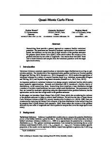
This definition captures the notion of important dimensions and quasi Monte Carlo methods perform best on problems which have low effective dimension. Low discrepancy sequences have a particular property that can be exploited to take advantage of the most important dimensions of problem which has a low effective dimension. It turns out that low discrepancy points are more uniformly distributed for projections onto the lower coordinates. The higher dimensional projections tend not to be as uniformly dispersed unless the number of points is very large. The easiest way to illustrate this property is through an example. To this end, we have generated 400 low discrepancy points in the 25 dimensional hypercube [0, 1)25 . These points are known as Halton points. In the next four Figures we have projected these points onto specific two dimensional planes. Thus Figure 1 is a projection onto the first two dimensions. Note that these points seem to be well dispersed over the square. Figure is a projection onto dimensions five and six and we note that these points 16

are still reasonably well dispersed but there are regular patterns. The regularity gets worse for the projection of dimensions 12 and 13. In the case of the projection of dimensions 24 and 25 the high correlation between the points leads to large gaps in the coverage. This is a general feature of low discrepancy sequences(see Morokoff and Caflish(1995))

1

0.9

0.8

0.7

Y axis

0.6

0.5

0.4

0.3

0.2

0.1

0

0

0.1

0.2

0.3

0.4

0.5 X axis

0.6

0.7

0.8

0.9

Figure 1: 400 Halton points in [0, 1)25 : projection of dimensions 1 and 2

17

1

1

0.9

0.8

0.7

Y axis

0.6

0.5

0.4

0.3

0.2

0.1

0

0

0.1

0.2

0.3

0.4

0.5 X axis

0.6

0.7

0.8

0.9

Figure 2: 400 Halton points in [0, 1)25 : projection of dimensions 5 and 6

18

1

1

0.9

0.8

0.7

Y axis

0.6

0.5

0.4

0.3

0.2

0.1

0

0

0.1

0.2

0.3

0.4

0.5 X axis

0.6

0.7

0.8

0.9

Figure 3: 400 Halton points in [0, 1)25 : projection of dimensions 12 and 13

19

1

1

0.9

0.8

0.7

Y axis

0.6

0.5

0.4

0.3

0.2

0.1

0

0

0.1

0.2

0.3

0.4

0.5 X axis

0.6

0.7

0.8

0.9

Figure 4: 400 Halton points in [0, 1)25 : projection of dimensions 24 and 25

20

1

If we can arrange matters so that the most important dimensions of a problem are generating using the early coordinates of the low discrepancy numbers this will improve computational efficiency. Caflish Morokoff and Owen(1997) exploit this idea by using a Brownian bridge construction to simulate a Brownian path. Under this construction the early quasi random numbers have the most influence on the simulated path. These early coordinates have very good distributional properties. Acworth, Broadie and Glassermann(1998) use principal components analysis to isolate the most important dimensions and then use the early coordinates of the low discrepancy points to simulate the most important components. Both these approaches lead to a marked increase in the efficiency of the quasi Monte Carlo method. Imai and Tan(2002) also use the same idea to develop a method for computing stochastic integrals using quasi Monte Carlo method. Their method takes into account the specific structure of the integral. They show how to obtain a linear transformation of the input random variables that maximizes the contribution of the early dimensions and so we describe it as the linear transformation(LT) method. This transformation is derived by a judicious selection of the elements of an orthogonal matrix. They demonstrate that it leads to computational efficiencies. We can apply their method to the optimal portfolio selection problem since the portfolio selection problem(in the CGZ set up) involves computing the expectation of stochastic integrals.

5

Computing the Optimal Portfolio Weights

In this section we describe how to use the Imam and Tan(2002) linear transformation to obtain the optimal portfolio weights. As we have seen this involves the numerical computation evaluation of ν in the CGZ method. We first illustrate how to compute the expected value of stochastic integral. We employ the same assumptions as in section 3.1. There is only one source of uncertainty. The price of the risky asset follows geometric Brownian motion, the riskless rate follows a single factor Cox Ingersoll Ross process and the market price of risk follows an Ornstein Uhlenbeck process. The key random variables in the stochastic integral for optimal wealth are r and θ. Hence 21

we discretion the stochastic differential equations for the interest rate and the market price of risk. Given the initial values r0 and θ0 , we use the approximations

rn = rn−1 + µr (rn−1 ) ∆t + σr (rn−1 )

√

∆tzn ; n = 1, . . . , N, √ θn = θn−1 + µθ (θn−1 ) ∆t + σθ (θn−1 ) ∆tzn ; n = 1, . . . , N

where N is the number of time steps, ∆t is the size of a time step where ∆t =

(31) (32) T . N

z =

(z1 , . . . , zN )0 is a transformed normal vector 





z1  .    .  = A  .   zN



ε1 ..  .  

(33)

εN

where ε = (ε1 , . . . , εN )0 is the original normal vector from some low-discrepancy sequence. 



a11 · · · a1N  . ..  ..  A =  .. . .   = (A.1 , · · · A.N ) aN 1 · · · aN N an orthogonal matrix that transforms the original normal vector into another normal vector. The idea is to pick the elements of this orthogonal matrix A so as to maximize the contribution of the early dimensions. These will be generated using the first few components of ε

0

which have very good distributional properties. It is convenient to introduce some new notation by defining Dt as Dt =

Z t 1Z t 2 θs ds + θs dWt 2 0 0

and Rt as Rt =

Z t 0

rs ds.

With this notation the state price density is ½

ξt

Z t 1Z t 2 = ξ0 exp − θ des − θs dWs 2 0 s 0

= e−Dt

¾

(34) 22

since ξ0 = 1. The Lagrange multiplier y can be written in terms of D and R as (

y= where ρ =

α . α−1

)α−1

X0

(35)

E [e−ρ(RT +DT ) ]

Hence to compute this multiplier we need to compute the following expec-

tation.

h

E e−ρ(RT +DT )

i

We now show how to apply the Imam-Tan procedure to the evaluation of this expectation. We derive a linear approximation of the function Y = e−ρ(RT +DT ) . We expand the function 0

Y around a point ε0 = (ε01 , . . . , ε0N ) . Then, at any point ε = ε0 + ∆ε, the function Y can be approximated by ³

Y (ε) ≈ Y ε

0

´

¯ N X ∂Y ¯¯ + ¯ ∂εl ¯ l=1

Because

∆εl .

Ã

∂Y ∂RT ∂DT = e−ρ(RT +DT ) (−ρ) + ∂εl ∂εl ∂εl we pay attention to the term Since RT =

RT 0

rs ds ≈

³

NP −1 n=0

∂RT ∂εl

+

∂DT ∂εl

´

(36)

εl =ε0l

!

(37)

; l = 1, . . . , N .

rn ∆t in the discretized model, N −1 X ∂rn ∂RT ≈ ∆t ∂εl n=0 ∂εl

∂rn ;n ∂εl

= 0, . . . , N − 1 can be sequentially specified. Because r0 is constant then

∂r0 ∂εl

= 0 is

satisfied. At any time n; n = 1 . . . , N − 1 Ã

!

√ ∂rn ∂rn−1 ∂µr (rn−1 ) ∂σr (rn−1 ) √ = 1+ ∆t + ∆tzn + σr (rn−1 ) ∆tan,l ∂εl ∂εl ∂rn−1 ∂rn−1 =

√ ∂rn−1 βr (rn−1 , zt ) + σr (rn−1 ) ∆tan,l ∂εl 23

(38)

where

Ã

!

∂µr (rn−1 ) ∂σr (rn−1 ) √ βr (rn−1 , zn ) = 1 + ∆t + ∆tzn . ∂rn−1 ∂rn−1 Note

∂zn ∂εl

= an,l ; n, l = 1, . . . , N .

For the CIR model

∂µr (rn ) ∂rn

= −κr and

∂σr (rn ) ∂rn

First we set ε0 = (0, . . . , 0)0 . In this case,

−1

= − 12 σr rn 2

∂rn ∂εl

is a linear function of ai,l ; i = 1, . . . , n.

Consequently, RT is also a linear function ai,l ; i = 1, . . . , N − 1 In the same way, we can specify DT as a linear function of ai,l ; i = 1, . . . , N . Since Z T 1Z T 2 = θ des + θs dWs 2 0 s 0

DT

N −1 µ X

≈

n=0

√ 1 2 θn ∆t + θn ∆tzn+1 2

¶

(39)

then, ∂DT ∂εl

≈

N −1 X

(

n=0

=

N −1 X n=0

where k1 (θn , zn+1 ) = θn ∆t +

√

) ´ √ ∂θn ³ θn ∆t + ∆tzn+1 + θn ∆tan+1,l ∂εl

(

∂θn k1 (θn , zn+1 ) + k2 (θn ) an+1,l ∂εl

)

(40)

∆tzn+1 and k2 (θn ) = θn ∆t. When we set ε0 = (0, . . . , 0)0

both k1 and k2 become constant regardless of elements in the orthogonal matrix. Therefore, ∂DT ∂εl

becomes a linear function of ai,l ; i = 1, . . . , N Consequently,

∂RT ∂εl

T + ∂D is a linear function of ai,l ; i = 1, . . . , N if we set ε0 = (0, . . . , 0)0 . ∂εl

Thus, let d = (d1 , . . . , dN )0 denote the coefficient vector that satisfies Ã

∂DT ∂RT + ∂εl ∂εl

!

= ε0 =(0,....0)0

24

N X n=1

dn an,l = (d · Al )

(41)

where Al is the l-th column vector of the orthogonal matrix, (a · b) represents an inner product between the vector a and b. Then Equation (36) can be written by ³

´

N

X 0 0 Y (ε) ≈ Y ε0 − ρe−ρ(RT (ε )+DT (ε )) (d · Al ) ∆εl

(42)

l=1

We can choose the orthogonal matrix in order to minimize the effective dimension of the function Y . For this purpose we choose the column vectors A.l step by step to minimize the effective dimension. The contribution to the total variance of Y arising from ∆ε1 is proportional to à N X

!2

dn an,1

n=1

If we select the elements of A.1 to maximize this expression, subject to the condition kA.1 k = 1. the optimal solution is A∗.1 = ±

d kdk

Since the matrix A must be orthogonal the following equation must be satisfied. (A.1 · A.l ) = 0; l = 2, . . . , N.

(43)

In order to specify the second row vector of the orthogonal matrix we change the pivotal point ε0 expansion. The point should be specified to incorporate the values of the first row vector A1 . Therefore, we set ε0 = (1, 0, . . . , 0)0 . In a similar way, we can specify the second row vector A2 . Because the A2 does not hold the orthogonality with the previous A∗1 , A∗2 must be adjusted by the Gram-Schmidt orthogonalization method. By changing the point to expand, we can specify all the elements of the orthogonal matrix A sequentially.

6

Computing the Optimal Weights

This section describes the direct procedure to compute Equation(29) at time zero using the LT method. One of the advantages of this procedure for the LT method is that we only 25

compute one matrix. Let U be the function in this expectation. Then, 1 U = √ {H∆t,T XT − X0 } z1 ∆t 1 = √ (CVT − X0 ) z1 ∆t

(44)

where C = er0 ∆t+(ρ−1)δT y ρ−1 is a constant, and VT = e−ρ(RT +DT )+D∆t is a function of ε. We think of a linear approximation of the function U . "

#

∂U 1 ∂VT =√ Cz1 + (CVT − X0 ) a1,l ; l = 1, . . . .N ∂εl ∂εl ∆t where

(

Ã

∂VT ∂DT ∂RT = VT −ρ + ∂εl ∂εl ∂εl

!

(45)

)

√

+ θ0 ∆ta1,l

(46)

Consequently, ∂U ∂εl

"

(

Ã

1 ∂RT ∂DT = √ Cz1 VT −ρ + ∂εl ∂εl ∆t "

Ã

∂DT 1 ∂RT + = √ −ρCVT z1 ∂εl ∂εl ∆t

!

!

)

√

#

+ θ0 ∆ta1,l + (CVT − X0 ) a1,l n

³

√

´

o

#

+ CVT θ0 ∆tz1 + 1 − X0 a1,l

(47)

Note if we set ε0 = (0, . . . , 0)0 , it leads to z1 = 0. ¯

∂U ¯¯ 1 √ {CVT − X0 } a1,l ¯ = ∂εl ¯ε=ε0 ∆t Therefore, the optimal solution of the first row vector of the orthogonal matrix is A∗1 = (1, 0, . . . , 0)0 . From a computational point of view, the second way to get the volatility term is more favourable. For the LT method, we can make use of the procedure of finding the Lagrange multiplier for computing the volatility. We use the same parameter values as in Cvitanic, Goukasian, and Zapater(2001).

26

Table 1: Base case parameter values

Parameter r¯ σr κr θ¯ σθ κθ r(0) θ(0) σS

Value = 0.0600 = 0.0364 0.0824 0.0871 0.0871 0.2100 0.0600 0.1000 0.2000

We first examine the case when T = 1 Table 1: Computing π with Monte Carlo α 0.5

CGZ 1.095

-1

0.252

-2

0.175

-5

0.110

-10 0.059

random1 1.103466 (0.01699) 0.262031 (0.00552) 0.18939 (0.00734) 0.119781 (0.009282) 0.089079 (0.009845)

random2 LD LD+LT 1.124985 1.131009 1.13119 (0.002912) (0.014338) (0.00158) 0.255412 0.252906 0.25331 (9.958e-4) (0.004642) (7.124e-4) 0.18103 0.1778935 0.17764 (0.001293) (0.006028) (9.230e-4) 0.109861 0.1061448 0.105849 (0.001581) (0.007354) (5.764e-4) 0.078501 0.0074545 0.074203 (0.001709) (0.007939) (6.179e-4)

In both LD and LD+LT, Latin-Supercube-Sampling is used that is based on 50-dimensional Sobol sequence. This means that, in 100-dimensional problem, we use two sets of permutations for scrambling the order of the original sequence. The number of time steps is N = 100, where ∆t =

T . N

As a set of simulation, we use from integer 0 to 215 − 1 to create the Sobol

sequence, and we repeat 10 replications to estimate the standard errors. For the comparison purposes we use the same procedure for computing the Lagrange multiplier with random sequences. The value of π is computing the direct procedure. In random1 we use 215 integers as a one set while we use 220 integers in random2. Both of theses are repeated 10 times. The 27

combination of low discrepancy sequences and the Imam Tan linear transformation method produces the lowest standard error. The improvement corresponds to a ten fold reduction in the standard error. Of course there is some extra work involved in obtaining the orthogonal matrix. In the next table, the time to maturity is changed to T = 5 which leads to N = 500 for the accurate discretization. In other words, we examine a 500-dimensional problem. Only first 23 columns of the orthogonal matrix are found for the LT method. The rest of the matrix is computed randomly. Table 2: Computing π with Monte Carlo(T = 5) α 0.5

CGZ 1.236

-1

0.295

-2

0.230

-5

0.170

-10 0.139

random1 random2 0.825050 1.223555 (0.35668) (0.02700) 0.32139 0.305848 (0.02025) (0.003708) 0.271348 0.251324 (0.02595) (0.004806) 0.225025 0.200594 (0.031195) (0.005861) 0.205045 0.178633 (0.03343) (0.006327)

LD LD+LT 1.6211524 1.222703 (0.289835) (0.034740) 0.3120086 0.304723 (0.013527) (9.211e-4) 0.2592218 0.2503222 (0.017345) (0.001232) 0.2097899 0.1977201 (0.021039) (0.002321) 0.1882696 0.1763573 (0.022688) (0.002179)

In both LD and LD+LT, Latin-Supercube-Sampling is used that is based on 50-dimensional Sobol sequence. This means that, in 500-dimensional problem, we use ten sets of permutations for scrambling the order of the original sequence. The number of time steps is N = 500, where ∆t =

T . N

As a set of simulation, we use from integer 0 to 215 − 1 to create the Sobol

sequence, and we repeat 10 replications to estimate the The value of π is computing the direct procedure. In random1 we use 215 integers as one set while we use 220 integers in random2. Both of them are repeated 10 times. The combination of low discrepancy sequences and the Imam Tan linear transformation method produces the lowest standard error. The improvement is again around a ten fold reduction in the standard error.

28

7

Summary

This paper discussed how Monte Carlo methods can be used to compute the optimal portfolio weights in the asset allocation problem if we can assume a complete market. We noted that the linear transformation method proposed by Imam and Tan(2002) significantly improves the efficiency of quasi Monte carlo methods in this connection. It would be interesting to apply this method to the procedure advocated by Detemple Garcia and Rindisbacher(2002. Based on standard Monte Carlo methods Detemple Garcia and Rindisbacher conclude that their method is more efficient than the CGZ procedure. It seems certain the approach developed in this paper will lead to improvements in the efficiency of the DGR method. This paper has concentrated on just one aspect of the asset allocation decisions. We have focussed on the numerical computation of the optimal asset mix assuming the input distributions and their parameters are known in a complete market setting. There are many other important dimensions of the asset allocation problem that we do not discuss. The incomplete market case is much harder: for work in this area Uppal and Kogin(2002) and Schachermayer. We have also not considered the modelling the input distributions and the attendant econometric issues. Our model assumes that the investor knows precisely the true distribution of the asset returns and the relevant state variables. Uppal and Wang(2002) have developed a model where the asset price dynamics are subject to ambiguity. It would also be of interest to explore the impact of constraints on the optimal asset mix. It is clear there are many possibilities for future research.

29

References Acworth P., M. Broadie, and P. Glasserman.(1998) A comparison of some Monte Carlo and quasi-Monte Carlo methods for option pricing. In Niederreiter, Hellekale, Larcher and Zinterhof Arrow, K.(1952) Le rˆ ole des valeurs boursi`eres pour la repartition meilleure des risques. Econometrie. Colloq. Internat. du CNRS, Paris, 40, 41-47 (with discussion, 47-48). English translation in Review od Economic Studies 31(1964) 91-96. Boyle P.P., M. Broadie, and P. Glasserman.(1997) Monte Carlo methods for security pricing. Journal of Economic Dynamics and Control, 21:1267–1321. Boyle, P., W. Tian and Fred Guan(2002): “ The Riccati Equation in Mathematical Finance,” Journal of Symbolic Computation, Vol 33, 3, 343-356. Brennan M., and Y Xia(2000), “ Stochastic Interest Rates and the Bond Stock Mix,” The European Finance Review, 4, 197-201. Brandt, M., A Goyal and P. Santa Clara(2001), ”A Simulation Approach to Dynamic Portfolio Choice with an Application to Industry Momentums’,Working Paper, Wharton School Caflisch R.E.,, W. Morokoff, and A. Owen(1997) Valuation of mortgage-backed securities using Brownian bridges to reduce effective dimension. Journal of Computational Finance, 1(1):27–46. Canner N., N. G. Manjow, and D. N. Weil(1997) An Asset Allocation Puzzle American Economic Review, 87:181-191. Cox, J. C. and Chi-fu Huang(1989) Optimum consumption and portfolio policies when asset prices follw a diffusuion process Journal of Economic Theory, 49:33–83. Cox, J. C.,J. Ingersoll and S. Ross(1985) A theory of the term structure of interest rates Econometrica , 53:385–408. Cvitanic J., Goukasian L., and F. Zapatero(2001), Monte Carlo Computaion of Optimal Portfolis in Complete Markets Working Paper, Dept of Mathematics UCLAe

30

Detemple, J. B, R. Garcia and M. Rindisbacher(2002),” A Monte carlo Method for Optimal Portfolios,” forthcoming Journal of Finance. Faure H,(1982), Discr´epance de suites associ´ees `a un syst`eme de num´eration (en dimension s). Acta Arithmetica, 41:337–351. Halton, J.H.,(1960) On the efficiency of certain quasi-random sequences of points in evaluating multi-dimensional integrals. Numerische Mathematik, 2:84–90, 1960. Imai, J. and K. Tan(2002), A method for reducing the effective dimension with applications to derivative pricing Working Paper, Dept of Mathematics, University of Waterloo. Joy,C., P.P. Boyle, and K.S. Tan(1996) Quasi-Monte Carlo methods in numerical finance. Management Science, 42(6):926–938. Karatzas, I., Lehoczky J.P., and S.Shreve(1987) Optimum portfolio and consumption decisions for a small investor on a finite horiozon SIAM Journal of Control and Optimization, 25:1557–1586. Karatzas, I., and S.Shreve(1998) Methods of Mathematical Finance Springer Verlag New York Karatzas, I., and S.Shreve(1991) Brownian Motion and Stochastic Calculus Springer Verlag New York Kim T.S. and E. Omberg(1996) Dynmaic Nonmyopic portfoli behavior Review of Financial Studies, 9:141–161. Liu J.(2001) Portfolio selection in stochastic environments Working Paper UCLA Markowitz, H.,(1952) Porfolio Selection Journal of Finance, 7:77-91. Merton R.C.,(1969) Lifetime portfolio selection under uncertainty: The continuous time case, Review of Economics and Statistics , 51:247–257. Merton R.C.,(1971) Optimum consumption and portfolio rules in a continuous time model Journal of Economic Theory,3:273–413. Morokoff, W., and R. E. and Caflisch(1994) Quasi random sequences and their discrepancy SIAM Journal of Scientific Computing , 15:1251–1270. 31

Niederreiter, H.,(1987) Point sets and sequences with small discrepancy. Monatshefte fur Mathematik, 104:273–337. Niederreiter, H.,(1992) Random Number Generation and Quasi-Monte Carlo Methods. S.I.A.M., Philadelphia, 1992. Ninomiya, S. and S. Tezuka(1996) Toward real-time pricing of complex financial derivatives. Applied Mathematical Finance, 3:1–20. Owen, A.(2001) The dimension distribution and quadrature test functions Working Paper, dept of Stistis Stanford University Paskov S.,and J.F. Traub. Faster Valuation of Financial Derivatives. Journal of Portfolio Management, 22(1):113–120. Pliska, S.(1986) A stochastic calculus model of continuous trading Mathemtics of Operations Research , 11:371–383. Sobol’, I.M.,(1967) The distribution of points in a cube and the approximate evaluation of integrals. U.S.S.R Computational Mathematics and Mathematical Physics, 7(4):86– 112, 1967. Uppal R., and T. Wang(2002) Model Misspecification and Under Diversification Working Paper , London Business School Wachter J.(2002) Portfolio and consumption decisions under mean reverting returns: an exact solution for complete markets. Forthcoming Journal of Financial and Quantitative Analysis.

32