and Seo (1995). Numerical integration is carried out from a state of rest on January 1, 1985, to December 31, 1994. The model analysis is performed beginning ...
Journal of Oceanography, Vol. 55, pp. 53 to 64. 1999
Assimilation of TOPEX/POSEIDON Altimeter Data with a Reduced Gravity Model of the Japan Sea NAOKI HIROSE1*, ICHIRO FUKUMORI2 and JONG-HWAN YOON 3 1Interdisciplinary
Graduate School of Engineering Sciences, Kyushu University, Kasuga 816-8580, Japan 2Jet Propulsion Laboratory, California Institute of Technology, Pasadena, CA 91109, U.S.A. 3Research Institute for Applied Mechanics, Kyushu University, Kasuga 816-8580, Japan (Received 3 June 1998; in revised form 24 September 1998; accepted 13 October 1998)
Sea level data measured by TOPEX/POSEIDON over the Japan Sea from 1993 to 1994 is analyzed by assimilation using an approximate Kalman filter with a 1.5 layer (reducedgravity) shallow water model. The study aims to extract signals associated with the first baroclinic mode and to determine the extent of its significance. The assimilation dramatically improves the model south of the Polar Front where as much as 20 cm2 of the observed sea level variance can be accounted for. In comparison, little variability in the northern cold water region is found consistent with the model dynamics, possibly due to significant differences in stratification.
1. Introduction In a recent study, Kim and Yoon (1996), using a reduced gravity model, successfully simulated the seasonal changes of the upper circulation of the Japan Sea. Their results qualitatively agree with surface charts of currents in terms of separation of the western boundary current, formation of the Polar Front, and generation of the subpolar gyre. Reduced gravity models have frequently been employed in simulating surface circulation in the equatorial and subtropical oceans. In the Japan Sea, although there is a clear two layer structure in the warm current region where the Tsushima Warm Current flows, stratification is weak during winter in the cold current region, i.e., the northwestern part of the Japan Sea (e.g., Senjyu and Sudo, 1993). As a result, the skill of reduced gravity models in simulating the circulation may be limited. The present study formally examines the extent to which a wind-driven reduced gravity model can describe variations of the Japan Sea by combining the model with sea level measurements of TOPEX/POSEIDON (hereinafter T/ P) (Fu et al., 1994). To this end, we proceed from a theoretical interpretation of a simulation to a quantitative comparison and assimilation of altimeter data with the model. The assimilation is performed by an approximate Kalman filter (Fukumori and Malanotte-Rizzoli, 1995). The model/ data comparison is a necessary step in calibrating uncertainties of the model and data. The assimilation allows
extraction of the signals consistent with model dynamics (first baroclinic mode) and thereby testing of the model’s fidelity. The efficacies of assimilation in interpolating the observations are also of interest; Although altimetric measurements are continuous along satellite ground tracks, the distance between tracks (~300 km) is larger than typical scale of eddies (~100 km) in this area. Assimilation allows for the model to dynamically interpolate and extrapolate such sparse observations. This manuscript is organized as follows. In Section 2, corrections made to the T/P altimeter data are discussed. The model and assimilation method are described in Sections 3 and 4. Results of the assimilation are given in Section 4, and a summary and discussion are presented in Section 5. 2. TOPEX/POSEIDON Data Correction The data analyzed in this study is the merged geophysical data record (M-GDR) of TOPEX/POSEIDON (Fig. 1) from December 1992 to December 1994 corresponding to cycles 9 to 84. All standard corrections are applied except for oceanic tide correction. As far as model assimilation is concerned, direct effects on data of processes not simulated by a model (e.g., phenomena related to barotropic motion and/or baroclinic instability for the present model), termed model representation errors, are indistinguishable from measurement noise (Cohn, 1997). Measurement noise and representation error, for a lack of a better terminology, are referred to collectively as observation error or data error. Standard assimilation schemes assume observation errors to be temporally uncorrelated. While most observation errors of the present
*Research Fellow of the Japan Society for the Promotion of Science. 53 Copyright The Oceanographic Society of Japan.
Keywords: ⋅ Data assimilation, ⋅ Kalman filter, ⋅ TOPEX/ POSEIDON, ⋅ sea level, ⋅ Japan Sea, ⋅ reduced-gravity model.
Fig. 1. Positions of the TOPEX/POSEIDON merged geophysical data record (M-GDR). The dashed line denotes the 200 m isobath; Data located at depths shallower than 200 m are eliminated from the study due to limited accuracies of available tidal corrections.
problem may be reasonably approximated to be uncorrelated as such, narrow band representation errors may not, which for the wind-driven reduced gravity model include oceanic tides and steric sea level changes due to seasonal heating and cooling. Proper modifications to assimilation methods are required for such correlated errors (e.g., Gelb, 1974). Alternatively, such noise may be removed from the data prior to assimilation. Sufficient in situ measurements are lacking to directly determine seasonal changes of density profiles. On the other hand, estimates of surface heat flux can be used to evaluate the seasonal heating/cooling effects on sea level. Gill and Niiler (1973) suggest that, on the seasonal time scale, horizontal advection of heat at mid-latitudes away from western boundary currents are negligible. Therefore, to first approximation, effects of changing heat flux are local. Climatological monthly mean surface heat flux estimates of Hirose et al. (1996) are used to evaluate the seasonal expansion and contraction of the upper water column. Temperature changes are computed locally assuming that warming and cooling occur uniformly within the top 50 dbar. Temperature is integrated in time using the Comprehensive Ocean Atmosphere Data Set (COADS) values in March as the initial condition when the mixed layer is deep. Salinity is assumed to be constant (34.0 PSU). Figure 2 shows the resulting steric sea level difference 54
N. Hirose et al.
Fig. 2. Climatological steric height difference from September to March estimated from surface heat flux data. The contour interval is 1.0 cm.
Fig. 3. Spatially averaged sea level variances. The figure compares effects of applying various corrections (surface heating and cooling, tides) in reducing the T/P data variance.
between summer and winter. Differences exceeding 10 cm is seen in the southeastern warm current region of the Japan Sea, while values along the Siberian coast are less than 5 cm. Subtracting the estimated steric changes from T/P data reduces the sea level variance by 16.8 cm2 (Fig. 3).
Tidal signal in the data are removed by estimates from a tide model. Four different oceanic tide models were compared; University of Texas Center for Space Research version 3.0 (UT CSR3.0), University of Grenoble version 95.2, Colorado State University (Kantha2), and University of Tokyo Ocean Research Institute (ORI96) (see, for example, Shum et al., 1997 for details). Figure 4 shows data residual variability after subtracting different tidal estimates. The variability is larger in the south than in northern parts of the domain. A large difference among the corrections occurs near the Tatarski Strait; In particular, the Kantha2 model results in residuals larger
than the original data themselves. These differences illustrate the difficulty in estimating tides in shallow regions. The magnitude of residuals provide one measure of the tidal models’ overall accuracy; In this regard the ORI96 model is most skillful and is employed to correct for ocean tides in this study. The along track altimeter data were averaged into values every 31 km along the T/P orbit so as to minimize computational storage. The resulting total number of the data points within the domain is 237 with an average variance of 55.1 cm2.
Fig. 4. Residual sea level variability after removing tidal components computed by different global tide models; (a) UT CSR3.0, (b) Grenoble FES95.2, (c) CU Kantha2, and (d) ORI96. Values are root-mean-square and contour interval is 1.0 cm. The dotted mark indicates data positions. Spline interpolation is performed in drawing the contours. Assimilation of TOPEX/POSEIDON Altimeter Data with a Reduced Gravity Model of the Japan Sea
55
3. Numerical Simulation 3.1 Reduced gravity model A non-linear, 1.5 layer, reduced gravity model is employed in this study (cf. equations (1) to (3) of Kim and Yoon, 1996). The model is capable of simulating winddriven first baroclinic motions and instabilities induced by horizontal current shears. The model is written in spherical coordinates and uses the Arakawa C-grid. Temporal integration is performed by leap-frog time-stepping with an intermittent use of the Matsuno (1966) scheme. Relevant model parameters are summarized in Table 1. The model extends from 33°N to 52°N in latitude and from 126.5°E to 142.5°E in longitude, covering the entire
Table 1. Parameters used in the present model.
Japan Sea. The model resolution is 1/6° in latitude and longitude, and is sufficiently high to reasonably resolve the dominant eddies of the Japan Sea. No slip and no flux boundary conditions are applied along the coastal boundaries determined from ETOPO5. The inlet volume transport through the Tsushima Strait is prescribed to be 2.2 ± 0.35 Sv (1 Sv = 106 m3s–1), varying sinusoidally in time annually with maximum value attained in September. The outlet eastward transport through the Tsugaru Strait is held constant (1.4 Sv) and a simple radiation condition is applied in the Soya Strait. These transports through the straits are consistent with values based on recent ADCP measurements (Isobe, 1994; Shikama, 1994). The model is also driven by daily wind forcing of Na and Seo (1995). Numerical integration is carried out from a state of rest on January 1, 1985, to December 31, 1994. The model analysis is performed beginning December 1992; The first eight years of the integration is considered a spinup period. 3.2 Results of the simulation The average and root-mean-square (rms) variability of the interface displacement from 1993 to 1994 are shown in Fig. 5. Contours of displacement may also be regarded as stream function under the geostrophic relation. Characteristic features of the upper circulation of the Japan Sea are found in the mean field; the East Korean Warm Current (EKWC), the Polar Front and the subpolar gyre. However,
Fig. 5. Interface displacement of the two year (1993 and 1994) mean (a) and its standard deviation (b). Contour intervals are (a) 5 m and (b) 2.5 m. The areal mean rms variability is 12.7 m. 56
N. Hirose et al.
the Tsushima Current along the Japanese coast is not evident due to the model’s lack of bottom topography. The EKWC displays overshooting to the north, but the cause is unclear. Strong variabilities are found south of the Polar Front and near the center of the subpolar gyre. The former is due to eddy activities and the latter corresponds to the seasonal variation of the cyclonic gyre. Model sea surface height anomaly η1(t) is related to interface displacement η(t) by,
η1 (t ) =
Fig. 6. Correlation between simulated sea level anomalies and TOPEX/POSEIDON altimeter data as a function of the model’s reduced gravity g′.
g′ ( η (t ) − η ), g
(1)
where η is the mean state of the interface displacement, g′ and g are the reduced and real gravitational accelerations, respectively. The sensitivity of the model to g′ is summarized in Fig. 6, which shows the correlation between T/P data and the simulated sea surface height anomaly as a function of g′. Although small, the simulation has maximum correlation with T/P for g′ = 2.33 cm s–2, and is used throughout this study. Figure 7(a) shows the spatial dependence of the correlation. Correlation between T/P and model simulation is small over most of the domain with an overall average value of 0.036. The statistical significance level of a correlation ra is (Bendat and Piersol, 1971),
Fig. 7. Correlation between TOPEX/POSEIDON altimeter data and simulated (a), assimilated (b), and forecasted (c) sea level anomalies. Contour interval is 0.1. The dotted mark indicates the data position. Assimilation of TOPEX/POSEIDON Altimeter Data with a Reduced Gravity Model of the Japan Sea
57
Fig. 8. Sea level variance accounted for by the simulation (a), assimilation (b), and 10-day forecasts (c). Contour interval is 5.0 cm2. Shaded areas denote regions where variance of model-data difference is larger than the data variance. The dotted mark indicates the data position.
ra =
2zα / 2 ec − 1 , where c = , c e +1 N −3
(2)
zα/2 is the 100 × α/2 percentage point of the standardized normal variable, and N is the number of degrees of freedom. zα/2 is 1.96 at 95% confidence, and N is 76 for the present analysis reflecting the number of data at individual observation points. Then, ra = 0.225, meaning that correlations smaller than this value are statistically indistinguishable from zero at the 95% confidence level. We must therefore conclude that the simulation has negligible correlation with T/P data over most of the domain. Figure 8(a) shows the spatial variation of the observed T/P sea level variance accounted for by the simulation. Explained variance is defined as data variance minus the variance of the model-data differences, viz., zTz – (z – Hx)T (z – Hx), where z denotes observations and Hx is the model’s equivalent of the observations (see, for example, Fu et al., 1993). Negative values indicate that there are more differences in model and data than similarities between the two. The negative explained variance and the small correlation found in most regions could be due to errors dominating the model estimate (and data). Quantification of such errors and testing the consistency between model and data are accomplished by data assimilation and are discussed in the following section. 58
N. Hirose et al.
4. Data Assimilation 4.1 The approximate Kalman filter The Kalman filter is a sequential estimation method that combines data and models minimizing the expected uncertainty of the solution. Direct application of Kalman filtering to ocean models analyzing real observations had largely been limited in the past due to the filter’s large computational requirements. In recent years, however, several approximations have been put forth that approximate the filter derivation, enabling near-optimal estimation using sophisticated ocean general circulation models. In this study, we will employ one of such approximations, the reducedstate filter of Fukumori and Malanotte-Rizzoli (1995). By approximating the model state, the reduced-state filter evaluates the model state error covariance matrix with fewer degrees of freedom than the model itself. The present model state vector x(t) can be expressed as, η (t ) x ( t ) = u( t ) v (t )
( 3)
where η(t) is the interface displacement and u(t) and v(t) are the velocity components. (Bold lower case letters denote
column vectors, with individual elements being one of the state variables at particular grid points. Bold upper case letters will denote matrices.) The reduced state approximation is established by defining a transformation, x (t ) ≈ Bx′ (t ) + x
( 4)
where x′ is a state vector of smaller dimension than x. Matrix B along with the reference state x are prescribed and together define the linear transformation. In this study, both B and x are time-invariant, and the latter is chosen to be the simulation’s time-mean state. The reduced state x′ was defined on a coarse 1 degree grid as shown in Fig. 9. Considering the dominant geostrophic balance, grid points of the reduced-state velocity are arranged between displacement points in the form of the Arakawa D-grid. Transformation from the coarse grid to the model’s original grid is performed by objective mapping (Bretherton et al., 1976) using a Gaussian correlation function with a 100 km decorrelation scale. Given the reduced state approximation, the model state’s error covariance matrix P(t) can be approximated in terms of the coarse state’s error P′(t) as,
P (t ) ≈ BP′ (t ) BT .
( 5)
The prime (′) indicates the reduced state and superscript T denotes matrix transpose. Evaluating P′ requires less computational resources than that of P, owing to the former’s smaller dimension. The Kalman gain matrix is then approximated by,
K (t ) = P (t ) H T (t ) R −1 (t ) ≈ BP′ (t ) BT H (t )T R −1 (t ) ( 6 ) where H(t) is the observation matrix such that Hx defines the model’s equivalent of the observations. Matrix R(t) is the data error covariance matrix and the superscript –1 denotes matrix inversion. The system matrices in the reduced state, which include the so-called state transition matrix, forcing matrix and observation matrix, are constructed numerically linearizing the model about the simulation’s mean state (Fukumori et al., 1993). In addition to the reduced-state approximation, a timeasymptotic approximation of the error covariance is employed to further reduce the computational requirements of Kalman filtering (Fukumori et al., 1993). The error covariance matrix often attains a near steady-state when observations are regularly assimilated. Approximating the error by such limit dramatically reduces the storage and the amount of computation associated with Kalman filtering (Anderson and Moore, 1979). Note that while P′ is approximated as time-invariant in Eq. (6), H and R are not. The limit of P′ is computed based
Fig. 9. Coarse grid on which the approximate Kalman filter is derived. State components η′, u′ and v′ are defined on +, 䊊 and 䊉, respectively. The total number of variables on the coarse grid is 310.
on the Riccati Equation. See Subsection 4.2 and Fukumori (1995) for specifies on computing such limit. Strictly speaking, although the true model state error P′ will not exactly become time-invariant (due to time-varing H, R etc.), we contend that such error limit based on the Riccati Equation (as well as the consequences of a reducedstate approximation) is closer to the true error than what could be obtained by merely guessing a P′. Given our inaccurate knowledge of model and data errors, the estimated P′ is practically indistinguishable from the truth. The validity of such ascertion is discussed in Subsection 4.3. It should also be noted that the approximations above are applied only in deriving the Kalman filter. The forward model retains its original resolution and temporal integration. 4.2 Estimation of errors Following Fu et al. (1993), data and model simulation error covariances can be estimated by,
{
R = < ( z − Hxsim )( z − Hxsim ) > T
}
− < Hxsim ( Hxsim ) > + < zz T > 2 T
Assimilation of TOPEX/POSEIDON Altimeter Data with a Reduced Gravity Model of the Japan Sea
( 7)
59
{
HP sim H T = < ( z− Hx sim )( z− Hx sim ) > T
}
+ < Hx sim ( Hx sim ) > − < zzT > 2 T
( 8)
where subscript sim denotes the simulation and z is the observations. The right-hand-side of Eqs. (7) and (8) can be evaluated by substituting observations and results of a simulation, replacing ensemble averages (angled brackets) with spatial and/or temporal means. For the present study, the averages were performed over space and time, assuming a spatially homogeneous and time-independent error. The resulting data and model (sea level) simulation error estimates are 54.1 and 9.1 cm2, respectively. These estimates are respectively close to data and model variabilities themselves (55.1 and 10.1 cm2 ), reflecting the low correlation between model simulation and T/P observations (Fig. 7). Estimates provided by Eqs. (7) and (8) are crude given the underlying approximations, and are later adjusted to achieve a consistent solution by the assimilation as described in the next subsection; The adjusted estimates for data and model simulation errors are 52.4 and 9.3 cm2, respectively. The data error covariance R is the sum of the altimeter’s instrument error and representation error (Section 2). The instrument error of the altimeter is modeled by a Gaussian covariance function with a 23.65 cm2 variance and a 1300 km e-folding scale measured along satellite ground tracks (Fukumori, 1995). The remainder of R (28.75 cm2) is regarded as contributions from missing model physics
(barotropic motion, baroclinic instability, etc.) and is treated as being spatially uncorrelated. Model process noise, i.e., the incremental error of model integration, is assumed to be time-invariant, and for simplicity is modeled in the form of wind forcing. The magnitude of process noise is adjusted so that the simulation error estimate based on the Lyapunov equation agrees with that obtained from Eq. (8). Such calibration results in an equivalent wind forcing error of 0.285 dyne2cm–4 with a decorrelation scale of 1-day. An asymptotic steady error covariance matrix P′ is finally obtained by integrating the Riccati equation, using time-invariant error covariances R and Q obtained above. In deriving the asymptotic limit of P′, observations are assumed to be available over the entire region (Fig. 1) instantaneously every 10 days, i.e., H is approximated as being time-invariant in the derivation of P′. The resulting estimate of P′ has a diagonal average of 28.0 m2 and 4.69 cm2 s–2 for displacement and horizontal velocities, respectively. The assimilation in effect reduces the model’s error variances without assimilation (i.e., simulation) in half. 4.3 Results of the assimilation Along-track T/P data from December 1992 to December 1994 are directly assimilated into the model. For simplicity, assimilation is performed every twenty-four hours at noon Japan Standard Time using all data measured within twelve hours of this instant, assuming the observations are coincident in time. Temporal anomalies of altimetric sea
Fig. 10. Model interface displacement on August 1, 1993; (a) simulation, (b) assimilation. Contour interval is 5 m. 60
N. Hirose et al.
level is assimilated as corresponding anomalies in the model; Equivalently, the model’s time-mean sea level is used in place of the unknown altimetric mean sea level. Figure 10 shows an example comparing results of the assimilation with that of the simulation. The two estimates of interface displacement are different in terms of the positions and radii of eddies and the meanders of the Polar Front. Subsurface temperature coinciding with this period was measured at CTD stations and is shown in Fig. 11. A warm eddy is detected at 200 m depth near 38.5 °N, 134°E (labeled A), which corresponds well with the deepening of the model interface resolved in the assimilation labeled A′. Additional supporting evidence of the same eddy was obtained during the CREAMS (Circulation Research of the East Asian Marginal Seas) summer cruise. At the same time, the negative anomaly labeled B′ in the assimilated estimate is suggestive of the cold anomaly, labeled B, in the hydrographic survey. The comparison between the assimilation and hydrographic survey demonstrates an example of detecting subsurface information from satellite altimetry. Correlation between assimilated estimate and T/P data increases to 0.294 on average, improving from that of the simulation almost everywhere (Fig. 7b). Higher correlation from 0.2 to 0.5 is found south of the Polar Front, where the model also explains as much as 20 cm2 of the observed sea level variance. The skill of the model as revealed by the assimilation demonstrates the significance of the first baroclinic mode. In fact, large density differences between the upper Tsushima Warm Current water and the lower cold Japan Sea Proper Water characterizes the hydrography south of the Polar Front, and strong baroclinicity have frequently been reported associated with meso-scale eddies
and EKWC (e.g., Naganuma, 1977; Yoon, 1991). The assimilation in effect quantifies the dominance of the first baroclinic mode. On the other hand, there are hardly any signal detectable consistent between model and altimetric observations in the cold water region. Over most of the northern region, correlation between assimilated estimate and T/P data is insignificant and the model explained data variance is negative. The lack of skill in the region may be explained by the weak stratification limiting the relative significance of baroclinic modes. Barotropic rather than baroclinic variability may dominate this area. Model-data correlation and model explained variance are also negative along the Japanese coast and near the North Korean Bay, which may reflect defects of the model. In particular, the Tsushima Current along the Japanese coast is lacking from the model and the EKWC overshoots as shown in Fig. 5(a). Figure 12 shows a longitude versus time plot of interface displacement along 38.5°N for the simulation and assimilation. Anomalies generally propagate westward as planetary Rossby waves, but assimilated estimates are sometimes stationary or are damped faster than in simulated results. Apparently, evolution of eddies are not as monotonic as the simulation suggests. Figure 13 is a similar diagram as Fig. 12 but along 130.5°E. In the simulation, anomalies propagate northward up to the Polar Front located at 39°N. Eddies may further be advected northward by the EKWC in this area, which can be partly confirmed in the assimilation. It should be noted that the temporal and spatial scales of the model’s motions are limited by the model’s resolution. Figures 12 and 13 show that the dominant scales are larger than 100 km in space and longer than 100 days in time.
Fig. 11. Subsurface temperature based on measurements made by CTDs and XBTs from July 23 to August 7, 1993. The observation points are shown by dotted marks. Contour interval is 1°C. Assimilation of TOPEX/POSEIDON Altimeter Data with a Reduced Gravity Model of the Japan Sea
61
Fig. 12. Interface displacement anomaly (η(t) – η ) for the simulation (a) and assimilation (b) along 38.5°N as a function of time. Time is shown in year day from January 1, 1993. Contour interval is 10 m. The shaded area shows negative anomalies.
The time step of the numerical integration is sufficiently small (30 min) compared to this scale, but the model’s spatial resolution of 1/6° is not. The grid resolution is apparently the limiting factor in the model’s ability to simulate smaller scales than those in Figs. 12 and 13. Posterior consistency checks are required to assure assumptions underlying the assimilation are sensible. One measure is provided by comparing model-data differences of the assimilation to their expected values;
< ( z− Hx ( − ))( z− Hx ( − )) >= R + HP ( − ) H T T
< ( z− Hx )( z− Hx ) >= R − HPH T . T
(9)
(10 )
The minus sign (–) denotes estimates immediately prior to the recursive assimilation of the observations. It was found that initial guesses of R and Q based on Eqs. (7) and (8) give slightly inconsistent residual estimates in Eqs. (9) and (10). After some trial and error, a consistent estimate was achieved by data and process noise estimates of 52.4 cm2 and 0.285 dyne2 cm–4, respectively (Subsection 4.2). All results pre62
N. Hirose et al.
sented above correspond to estimates based on these uncertainty estimates. 4.4 10-day forecasts Model estimates immediately prior to the recursive assimilation, x(t, –), represent forecasts. Although assimilation is performed at twenty-four hour intervals, the model integrated state x(t, –) can be considered a ten-day forecast because observations are only available at ten-day intervals at any given location. Figure 7(c) shows the correlation between sea levels of the forecasted state Hx(t, –) and the observations z(t). The spatial average of the correlation is 0.211. On the other hand, correlation between the filtered estimates and data ten days later is 0.201. This difference in correlation suggests the model having skill in propagating information in time from past observations. The model forecast retains much of the assimilation’s skill south of the Polar Front, demonstrating the model’s ability in forecasting variability in this area over ten days. Because the dominant time-scale of motion in this area is longer than 100 days, as discussed in the preceding subsection, it may be possible to numerically forecast vari-
Fig. 13. Same as Fig. 12 but along 130.5°E.
ability over a longer period than the 10-days considered here. 5. Summary and Discussion TOPEX/POSEIDON altimeter data were assimilated into a reduced gravity model of the Japan Sea to test the quantitative skill of the model’s dynamics. Temporally correlated variability due to oceanic tides and seasonal heating and cooling of the water column were removed from the T/P M-GDR prior to assimilation. Steric height changes due to seasonal heating and cooling were evaluated using estimates of surface heat flux. Annual steric height differences exceeding 10 cm are found in the southern region of the Japan Sea. Four different global tide models were compared in removing tidal components from T/P data; Among the four considered, the ORI96 model results in the smallest residual variability. However, although acceptable to first approximation, these corrections might not be accurate. Steric height changes should ideally be estimated from in-situ density observations or the study should employ more sophisticated models which can simulate changes in vertical stratification. The resolution of most tide models are also not sufficient to adequately simulate tide propagation in
marginal seas. A 1.5 layer (reduced-gravity) shallow water model of the Japan Sea was used in this study. The model was forced by daily winds and by prescribed inflow and outflow through the three straits. Although the model is able to qualitatively simulate the general pattern of the surface circulation, correlation with T/P data was statistically insignificant over most of the domain. Inaccuracies in external forcing and model numerics limits the skill of the simulation. An approximate Kalman filter was employed to extract signal in the data consistent with model dynamics through sequential assimilation. The signals associated with the first baroclinic modes and instabilities due to horizontal velocity shears are detectable in this assimilation, but the remaining signals such as barotropic motions and baroclinic instabilities are representation errors which constitutes a part of data error. The assimilation identifies a warm eddy north of the Polar Front in summer of 1993, which was validated by independent in-situ observations. In the Tsushima Warm Current region except near the Japanese coast, the model accounts for as much as 20 cm2 of the T/P data variance. This result demonstrates the significance of the first baroclinic mode in the region. On the other hand, the model explained
Assimilation of TOPEX/POSEIDON Altimeter Data with a Reduced Gravity Model of the Japan Sea
63
little variability of the data in the northern and coastal regions. It is speculated that other physics, such as the barotropic mode, dominate such regions. Errors of the assimilated state were estimated to be 5.3 m for interface displacement (1.3 cm for sea level anomaly) and 2.2 cm s–1 for horizontal velocity. The present assimilation could be improved in many ways. For example, spatial variations in data and model error covariances (R and Q) were not considered in this study. The model’s errors were modeled in the form of wind forcing, which may not fully account for other error sources, such as errors in the inflow and outflow conditions. The optimal smoother, which utilizes formally future observations in making estimates, may further improve the solution. These and other improvements will be considered in future studies. The 10-day forecast demonstrates a nontrivial skill of the model in the warm water region. It may be expected that numerical forecasting of the first baroclinic component in such region is possible for several tens of days. However, in actual forecasts, the skill is further limited by the availability and accuracy of future forcing fields (e.g., atmospheric forecasts, climatological winds). Acknowledgements Helpful comments by Prof. A. G. Ostrovskii and Mr. H. Hase (both at Kyushu University) are appreciated. The reduced-gravity model was originally written by Dr. C.-H. Kim (Korea Ocean Research Development Institute). Most of the computation was performed on the CRAY J-90 of the Jet Propulsion Laboratory (JPL) Supercomputing Project. The tide models and T/P M-GDR were provided by the Physical Oceanography Distributed Active Archive Center at JPL. The COADS data was supplied by the Japan Meteorological Agency. The CTD and XBT data were obtained from the Ocean Prompt Report (Maizuru Marine Observatory). The ETOPO5 data was distributed by National Geophysical Data Center. References Anderson, B. D. O. and J. B. Moore (1979): Optimal Filtering. Prentice-Hall, Englewood Cliffs, New Jersey, 357 pp. Bendat, J. S. and A. G. Piersol (1971): Random Data: Analysis and Measurement Procedures. Wiley-Interscience, New York, 407 pp. Bretherton, F. P., R. E. Davis and C. B. Fandry (1976): A technique for objective analysis and design of oceanographic experiments applied to MODE-73. Deep Sea Res., 23, 559– 582. Cohn, S. E. (1997): An introduction to estimation theory. J. Meteor. Soc. Japan, 75, 257–288.
64
N. Hirose et al.
Fu, L.-L., I. Fukumori and R. N. Miller (1993): Fitting dynamic models to the Geosat sea level observations in the Tropical Pacific Ocean, II, A linear, wind-driven model. J. Phys. Oceanogr., 23, 2162–2181. Fu, L.-L., E. J. Christensen, C. A. Yamarone, Jr., M. Lefebvre, Y. Ménard, M. Dorrer and P. Escudier (1994): TOPEX/ POSEIDON mission overview. J. Geophys. Res., 99, 24,369– 24,381. Fukumori, I. (1995): Assimilation of TOPEX sea level measurements with a reduced-gravity shallow water model of the tropical Pacific Ocean. J. Geophys. Res., 100, 25027–25039. Fukumori, I. and P. Malanotte-Rizzoli (1995): An approximate Kalman filter for ocean data assimilation: An example with an idealized Gulf Stream model. J. Geophys. Res., 100, 6777– 6793. Fukumori, I., J. Benveniste, C. Wunsch and D. B. Haidvogel (1993): Assimilation of sea surface topography into an ocean circulation model using a steady-state smoother. J. Phys. Oceanogr., 23, 1831–1855. Gelb, A. (1974): Applied Optimal Estimation. M.I.T. Press, Cambridge, MA, 374 pp. Gill, A. E. and P. P. Niiler (1973): The theory of the seasonal variability in the ocean. Deep Sea Res., 20, 141–177. Hirose, N., C.-H. Kim and J.-H. Yoon (1996): Heat budget in the Japan Sea. J. Oceanogr., 52, 553–574. Isobe, A. (1994): Tsushima Warm Current at Tsushima Straits. Kaiyo Monthly, 26, 802–809 (in Japanese). Kim, C.-H. and J.-H. Yoon (1996): Modeling of the wind-driven circulation in the Japan Sea using a reduced gravity model. J. Oceanogr., 52, 359–373. Matsuno, T. (1966): Numerical integrations of the primitive equations by a simulated backward difference method. J. Meteor. Soc. Japan, 44, 76–84. Na, J.-Y. and J.-W. Seo (1995): Comparison between the sea surface winds and the current measurements in the northern part of the East/Japan Sea. 8th PAMS & JECSS Workshop, Matsuyama, Japan, 82–87. Naganuma, K. (1977): The oceanographic fluctuations in the Japan Sea. Mar. Sci. (Kaiyo Kagaku), 9, 137–141 (in Japanese with English abstract). Senjyu, T. and H. Sudo (1993): Water characteristics and circulation of the upper portion of the Japan Sea Proper Water. J. Mar. Sys., 4, 349–362. Shikama, N. (1994): Current measurements in the Tsugaru Strait using bottom-mounted ADCPs. Kaiyo Monthly, 26, 815–818 (in Japanese). Shum, C. K., P. L. Woodworth, O. B. Andersen, G. D. Egbert, O. Francis, C. King, S. M. Klosko, C. Le Provost, X. Li, J.-M. Molines, M. E. Parke, R. D. Ray, M. G. Schlax, D. Stammer, C. C. Tierney, P. Vincent and C. I. Wunsch (1997): Accuracy assessment of recent ocean tide models. J. Geophys. Res., 11, 25173–25194. Yoon, J.-H. (1991): The seasonal variation of the East Korean Warm Current. Rep. Res. Inst. Appl. Mech. Kyushu University, 38, 23–36.