Association testing in bisulfite sequencing data via a. Laplace approximation: Supplementary Information. 1 Supplementary Figures. 0. 0.25. 0.5. 0.75. 1.
Association testing in bisulfite sequencing data via a Laplace approximation: Supplementary Information
Supplementary Figures
MALAX−2 MALAX−1g MALAX−1m MACAU BB
power
0.75
0.5
0.25
0
1
1
1
0.75
0.75
power
1
power
1
0.5
0.25
10−1
10−2
0
10−3
1
0.5
0.25
10−1
10−2
0
10−3
1
10−1
10−2
10−3
significance threshold
significance threshold
significance threshold
0% DM sites
25% DM sites
50% DM sites
Supplementary Figure S1: Power measures for the evaluated methods under various proportions of differentially methylated sites. All results are averaged over 10 simulated data sets.
% true positives
100
MALAX−1g GEE PQL
75
50
25
0
0
100
200
400
#top sites
400
500
Supplementary Figure S2: The detection power of MALAX-1g and two additional evaluated methods under simulated data sets with no DM sites. The additional methods are GEE (based on CARAT) and PQL (based on GMMAT), as described in the supplementary note. All results are averaged over 10 simulated data sets.
1
2
Experiments with Additional Methods
We evaluated two additional methods for generalized linear mixed model (GLMM) approximation. Both methods were recently proposed for case-control association studies, but can be readily adapted to work with count-bases responses instead of binary responses. The first method is based on the penalized quasi likelihood algorithm, as implemented in the GMMAT package [1]. This method is similar to the Laplace approximation but applies additional approximations, which results in faster computations at the cost of reduced accuracy. The second method uses a generalized estimating equations (GEE) approach, as implemented in the CARAT package [2]. This method only models the first two moments of the model likelihood. We used a modified version of CARAT that was adapted to use a binomial instead of a binary response. We evaluated both a standard version and a version with an additional dispersion parameter, as described in [2]; both versions yielded effectively the same results. GMMAT and CARAT were evaluated in a setting with no differentially methylated (DM) sites, which was the easiest setting in our experiments. Consequently, both methods used one variance component associated with a genetic similarity matrix, along with one variance component associated with the identity matrix, which can account for independent over-dispersion. The results demonstrate that MALAX-1g substantially outperformed both methods (Supplementary Figure S2). We therefore did not consider these methods in the remainder of the experiments. We note that we also evaluated versions of these approaches that use beta-binomial instead of binomial responses, but these versions were less accurate than the binomial ones.
3
Gradient Computation
The gradient of the approximate log likelihood described in the main text is required both for approximating the Hessian and for the maximum likelihood estimation procedure. Here we derive the gradient computation in detail. We first explicitly write the approximate log likelihood as follows: �
log P y j | x, W , r j
�
n � � X � � �T 1 �ˆ 1 l − m G−1 ˆl − m + log P yij | ˆli − log |B| , | 2 {z } i=1 |2 {z }
≈−
L1
|
{z
L2
}
L3
(1) where B , GA. We denote the three terms on the right hand side of the above equation as L1 , L2 and L3 , respectively. Note that the quantities G and m in L1 depend explicitly on the model parameters, but ˆl and A also implicitly depend on these parameters, where the dependence of A is mediated entirely through its dependence on ˆl. We therefore divide the partial derivative according to each parameter θ (which can represent variance components or fixed effects) into its explicit and implicit components, by using the chain rule as follows: � � n X ∂log P y j | x, W , r j ∂L1 ∂log P y j | x, W , r j ∂ ˆli = |explicit + . (2) ∂θ ∂θ ∂θ ∂ ˆli i=1 2
We first derive the explicit components: � i �T � 1 h ∂L1 1 �ˆ −1 −1 ˆ −1 | = − l − m G K G l − m − tr G K v v explicit ∂σv2 2 2 � � i � � h T 1 ˆ 1 ∂L1 −2 ˆ −1 | = − l − m G l − m − tr G explicit ∂σe2 2 2 � �T ∂L1 |explicit = − ˆl − m G−1 C. ∂γ
(3)
Here, C is the matrix of covariates for the entire sample (the matrix W with an appended h
column x), and γ = αT β
iT
is the vector of all fixed effects.
To derive the implicit components, we first note that ∂log|B| ∂ ˆ li ∂θ . ∂ˆ li
therefore only need to compute the negative Hessian A as follows: �
∂(L1 +L2 ) |l=ˆl ∂l
= 0 by definition. We
To derive log |B| , we first explicitly write
�
�
�
A , −∇∇log P l | x, W , y j , r j |l=ˆl = −∇∇log P y j | l |l=ˆl + G−1 . Using this explicit notation,
∂log|B| ∂ˆ li
"
#
is given by: "
∂log |B| ∂B 1 1 = − tr B −1 |l=ˆl = tr B −1 Gdiag 2 2 ∂ ˆli ∂ ˆli where
∂B ∂ˆ li
(4)
!#
� � ∂3 j log P y | l |l=ˆl ∂li3
,
(5)
is a matrix of element-wise partial derivatives.
�� ˆ Finally, ∂∂θli can be derived by using the fact that ˆl = G∇ log P y j | l |l=ˆl + m, as explained in the main text. Therefore, for every parameter θ we have: �� � � �� ∂ ∇ log P y j |l |l=ˆl ∂ˆl ∂ˆl ∂G � ∂m j = ∇ log P y | l |l=ˆl + G + , ∂θ ∂θ ∂θ ∂θ ∂ˆl
(6)
where the partial derivatives over matrices and vectors are computed element-wise. Writing these gradients explicitly for the model parameters, we have: � � �� � � �� ∂ˆl ∂ˆl j j = K ∇ log P y | l | + G∇∇ log P y | l | v ˆ ˆ l=l l=l ∂σ 2 ∂σv2 v � � � � � � � � ˆ ˆ ∂l ∂l = ∇ log P y j | l |l=ˆl + G∇∇ log P y j | l |l=ˆl 2 2 ∂σe ∂σe � � � � ˆ ˆ ∂l ∂l = G∇∇ log P y j | l |l=ˆl + Ck, ∂αk ∂αk
(7)
where C k is the k th column of C. A careful analysis reveals that the only matrix that needs to be inverted is B [3]. This is also the matrix whose determinant needs to be evaluated in the likelihood evaluation. Both quantities can be readily evaluated given the Cholesky decomposition of B, whose computation scales cubically with the sample size. Hence, gradient computation incurs only a minor additional computational overhead over the likelihood approximation.
3
4
Data Simulations
The simulations procedure consisted of several stages: Genotype simulations, covariates simulations, cell-type simulations, phenotype simulation, methylation simulations and observed reads simulations. We describe each stage in turn.
4.1
Genome simulations
We simulated population structure via the Balding-Nichols model [4], wherein allele frequencies in the range [0.05, 0.5] were randomly drawn for an ancestral population, and frequencies for several subpopulations were drawn from a Beta distribution with parameters f (1 − F ST ) /FST and (1 − f ) (1 − F ST ) /FST , where f is the minor allele frequency in the ancestral population. Next, we generated a mixture vector M i for every individual i from a symmetric DirichP let distribution with a concentration parameter 0.25, such that u M iu = 1, and u iterates over subpopulations. Finally, 60,000 SNPs were generated for every individual assuming Hardy-Weinberg equilibrium by sampling every SNP j of individual i from P Bin(2, pij ), where pij = u M iu fuj , and fuj is the MAF of SNP j in population u.
4.2
Covariate simulations
A vector of covariates for every individual i, C i , was generated by sampling each entry from a standard normal distribution, and adding an additional entry with the value 1.0 as an intercept.
4.3
Cell-type simulations
A vector of cell-types for every individual i, T i , was generated from a non-symmetric Dirichlet distribution with concentration parameters 1.33 , 0.93 , 4.299, 2.696, 16.344. These values were fitted using estimated cell type proportions for the GSE42861 dataset [5], a 450K array data set. Specifically, we obtained cell proportion estimates of five cell types (granulocytes, monocytes, B cells, NK cells, T cells) using the default implementation available in the minfi package [6], defined and assembled for the 450K array [7] based on the approach suggested by [8] and a 450K reference data set [9].
4.4
Phenotype simulation
To generate a phenotype, we first sampled effect sizes for the factors affecting the phe2 ) for every causal SNP notype. Specifically, we sampled an effect size γlsnp ∼ N (0, σsnp pop 2 l, an effect size γu ∼ N (0, σpop ) for every subpopulation u (intended to model shared 2 ) environmental factors within the subpopulations), and an effect size γhcell ∼ N (0, σcell for every cell-type h.
4
Afterwards, the phenotype y i for every individual i was generated as follows: sil γlsnp +
X
yi = +
X
miu γupop +
j
l∈Causal
X
tih γhcell + �i ,
(8)
h
where sil , miu and tih are the lth causal SNP, uth subpopulation ancestry fraction and hth cell-type fraction of individual i, respectively, �i ∼ N (0, σ�2 ) is an environmental effect for individual i where σ�2 guarantees that the phenotype variance is 1.0, and l iterates over indices of causal SNPs only. All effects were normalized to have a zero mean and unit variance.
4.5
Methylation simulation
Methylation levels πji for every site j of every individual i were generated as follows: First, either 0%, 25% or 50% of the sites were randomly selected to be differentially methylated. Next, for every site j we generated effect sizes for the factors affecting 2,j ) for every the methylation. Specifically, we sampled an effect size δkj,covar ∼ N (0, νcovar j,snp 2,j covariate k and site j, an effect size δl ∼ N (0, νsnp ) for every causal SNP l and site 2,j j,pop ∼ N (0, νpop ) for every subpopulation u and site j (intended to j, an effect size δu model shared environmental factors within the subpopulations), an effect size δhj,cell ∼ 2,j 2,j N (0, νcell ) for every cell-type h and site j, and an effect size δ j,pheno ∼ N (0, νpheno ) for i 2,j the phenotype. We also generated an environmental effect ej ∼ N (0, νenv ) for every site j of individual i. �
�
Next, we generated logit πji,h for every cell type h of site j of individual i as follows: �
�
logit πji,h =
X
cik δkk,covar +
k
sil δlj,snp +
X
X
miu δuj,pop + δhj,cell + y i δ j,pheno + eij .
u
l∈Causal
(9) In the next step, the methylation level of every cell type h of site j of individual i, πji,h , �
�
�
was computed as πji,h = 1/ 1 + exp −logit πji,h
���
. Finally, a combined methylation
level πji for every individual i of every site j was computed via: πji =
X
tih πji,h .
(10)
h
4.6
Observed reads simulation
To simulate observed reads, we first sampled a total number of reads rji for every site j of individual i from a negative Binomial distribution with parameters n = 1.135515, p = 0.047623. These values were fitted from the distribution of total number of reads of the Baboons data studied in the original MACAU paper [10]. Afterwards, an observed number of reads yji for every site j of individual i was sampled from Bin(rji , πji ).
5
4.7
Default parameters
Unless otherwise stated, the default parameters used in the simulations are the following: Each data set consisted of 200 individuals, 3 covariates (including an intercept), 60,000 SNPs, 500 causal SNPs, 10,000 non-causal sites and 500 causal sites. The ancestry of every individual was a mixture of four different populations, sampled from a symmetric Dirichlet distribution with concentration parameter of 0.25. Additionally, every individual contained a mixture of 5 cell types, sampled from a Dirichlet distribution with parameters 1.33 , 0.93 , 4.299, 2.696, 16.344. 2 2 The default effect variances were the following: σsnp = 0.25 / #SNPs, σpop = 0.025 / 2 2,j 2,j #populations, σcell = 0.25 / #cell-types, νcovar = 0.01 / #covariates, νsnp = 1 / #SNPs, 2,j 2,j = 0.1 / #populations, ν 2,j 2,j νpop pheno = 0.025, νenv = 0.1, νcell = 5.0.
References [1]
H. Chen et al. Control for Population Structure and Relatedness for Binary Traits in Genetic Association Studies via Logistic Mixed Models. Am. J. Hum. Genet. 98(4) (2016), 653–66.
[2]
D. Jiang, S. Zhong, and M.S. McPeek. Retrospective binary-trait association test elucidates genetic architecture of Crohn disease. Am. J. Hum. Genet. 98(2) (2016), 243–255.
[3]
C. Rasmussen and C. Williams. Gaussian Processes for Machine Learning. The MIT Press, 2006.
[4]
D.J. Balding and R.A. Nichols. A method for quantifying differentiation between populations at multi-allelic loci and its implications for investigating identity and paternity. Genetica 96(1-2) (1995), 3–12.
[5]
Y. Liu et al. Epigenome-wide association data implicate DNA methylation as an intermediary of genetic risk in rheumatoid arthritis. Nat. Biotechnol. 31(2) (2013), 142–147.
[6]
M.J. Aryee et al. Minfi: a flexible and comprehensive Bioconductor package for the analysis of Infinium DNA methylation microarrays. Bioinformatics 30(10) (2014), 1363–1369.
[7]
A.E. Jaffe and R.A. Irizarry. Accounting for cellular heterogeneity is critical in epigenome-wide association studies. Genome Biol. 15(2) (2014), 1.
[8]
E.A. Houseman et al. DNA methylation arrays as surrogate measures of cell mixture distribution. BMC Bioinform. 13(1) (2012), 1.
[9]
L.E. Reinius et al. Differential DNA methylation in purified human blood cells: implications for cell lineage and studies on disease susceptibility. PLOS ONE 7(7) (2012), e41361.
[10]
A.J. Lea, J. Tung, and X. Zhou. A Flexible, Efficient Binomial Mixed Model for Identifying Differential DNA Methylation in Bisulfite Sequencing Data. PLoS Genet. 11(11) (2015), e1005650.
6