Astronomy Astrophysics

Astronomy & Astrophysics

A&A 391, 195–212 (2002) DOI: 10.1051/0004-6361:20020612 c ESO 2002

Theoretical isochrones in several photometric systems I. Johnson-Cousins-Glass, HST/WFPC2, HST/NICMOS, Washington, and ESO Imaging Survey filter sets L. Girardi1,2 , G. Bertelli3,4 , A. Bressan4 , C. Chiosi1 , M. A. T. Groenewegen5,6 , P. Marigo1 , B. Salasnich1 , and A. Weiss7 1 2 3 4 5 6 7

Dipartimento di Astronomia, Università di Padova, Vicolo dell’Osservatorio 2, 35122 Padova, Italy Osservatorio Astronomico di Trieste, via Tiepolo 11, 34131 Trieste, Italy Istituto di Astrofisica Spaziale, CNR, via del Fosso del Cavaliere, 00133 Roma, Italy Osservatorio Astronomico di Padova, Vicolo dell’Osservatorio 5, 35122 Padova, Italy PACS ICC-team, Instituut voor Sterrenkunde, Celestijnenlaan 200B, 3001 Heverlee, Belgium European Southern Observatory, Karl-Schwarzschild-Str. 2, 85740 Garching bei München, Germany Max-Planck-Institut für Astrophysik, Karl-Schwarzschild-Str. 1, 85740 Garching bei München, Germany

Received 5 November 2001 / Accepted 19 April 2002 Abstract. We provide tables of theoretical isochrones in several photometric systems. To this aim, the following steps are

followed: (1) first, we re-write the formalism for converting synthetic stellar spectra into tables of bolometric corrections. The resulting formulas can be applied to any photometric system, provided that the zero-points are specified by means of either ABmag, STmag, VEGAmag, or a standard star system that includes well-known spectrophotometric standards. Interstellar absorption can be considered in a self-consistent way. (2) We assemble an extended and updated library of stellar intrinsic spectra. It is mostly based on “non-overshooting” ATLAS9 models, suitably extended to both low and high effective temperatures. This offers an excellent coverage of the parameter space of T eff , log g, and [M/H]. We briefly discuss the main uncertainties and points still deserving more improvement. (3) From the spectral library, we derive tables of bolometric corrections for JohnsonCousins-Glass, HST/WFPC2, HST/NICMOS, Washington, and ESO Imaging Survey systems (this latter consisting on the WFI, EMMI, and SOFI filter sets). (4) These tables are used to convert several sets of Padova isochrones into the corresponding absolute magnitudes and colours, thus providing a useful database for several astrophysical applications. All data files are made available in electronic form. Key words. stars: fundamental parameters – Hertzprung-Russell (HR) and C-M diagrams

1. Introduction One of the primary aims of stellar evolution theory is that of explaining the photometric data – e.g. colour-magnitude diagrams (CMDs), luminosity functions, colour histograms – of resolved stellar populations. To allow whatever comparison between theory and data, the basic output of stellar models – the surface luminosity L and effective temperature T eff – must be first converted into the observable quantities, i.e. magnitudes and colours. This conversion is performed by means of bolometric corrections (BC) and T eff -colour relations, and later by considering the proper distance, absorption and reddening of the observed population, and the photometric errors. Determining BCs and T eff -colour relations is indeed one of the most basic tasks in stellar astrophysics. Empirical determinations (see e.g. the compilations by Schmidt-Kaler 1982; Flower 1996; Alonso et al. 1999a,b) involve a great Send offprint requests to: L. Girardi, e-mail: [email protected]

observational effort, and are obviously the most reliable if compared to purely theoretical determinations. However, since the empirical calibrations are mostly based on nearby stars, only a limited region in the space of stellar parameters (T eff , log g, and metallicity [M/H]) can be covered by observations. This contrasts with our present-day capabilities of getting resolved photometry of populations that are certainly very different from the local one, like those in dwarf galaxies and in the Bulge. For instance, present empirical relations do not include young-metal poor populations, or super-metal rich stars, which are likely present in the resolved galaxies of the Local Group. Another important limitation of empirical relations is that they are usually available just for a small set of filters or photometric systems, like the popular Johnson-Cousins-Glass one. Again, this is in contrast with the rapid diffusion in the use of specific filter sets, for which no empirical relation is yet available, though large databases are already being collected. Just to mention a few relevant examples, new filter sets have been adopted in the Hubble Space Telescope (HST)

Article published by EDP Sciences and available at http://www.aanda.org or http://dx.doi.org/10.1051/0004-6361:20020612

196

L. Girardi et al.: Isochrones in several photometric systems

Wide Field Planetary Camera 2 (WFPC2), in the European Southern Observatory (ESO) Wide Field Imager (WFI), and in the Hipparcos mission. Moreover, brand-new photometric systems have been designed for the Sloan Digital Sky Survey (SDSS), and will be adopted in the future GAIA mission. An impressive amount of data will be provided by these instruments in the coming years, and much of it will soon become of public access. Then, it would be highly desirable to have the capability of converting stellar models to these many new photometric systems, bypassing for a moment the time-consuming procedure of empirical calibration. With this target in mind, we have undertaken a project aiming at providing theoretical BCs and colour transformations for any broad-band photometric system, and many intermediateband systems as well. Actually, the project starts with the work by Bertelli et al. (1994), who presented a large database of theoretical isochrones and converted them to the JohnsonCousins-Glass U BVRI JHK system. The transformations were primarily based on Kurucz (1993) synthetic atmosphere models, suitably extended in the intervals of lower and higher effective temperatures. In Chiosi et al. (1997), the same theoretical isochrones are converted to the WFPC2 photometric system, and the attention is paid to the features that isochrones and single stellar populations present in ultraviolet (UV) colours. In particular, they address the question whether the variation of UV colours of elliptical galaxies as a function of red-shift presents signatures from which one can infer the age and type of the source emitting the UV flux. Later on, Salasnich et al. (2000) present new isochrones for α-enhanced chemical mixtures, for both U BVRI JHK and WFPC2 photometric systems. The present work is a natural follow-up of this project, in which, besides extending the number of available photometric systems, we aim at updating and improving the database of stellar spectra which is at the basis of the complete procedure. The plan of this paper is as follows: Sect. 2 details the adopted formalism. In Sect. 3, we describe the stellar spectral library in use. Section 4 gives the basic information about the several photometric systems under consideration. The resulting tables of bolometric corrections are then applied to a large database of stellar isochrones, which are already described in published papers and briefly recalled in Sect. 5. Section 6 illustrates some main properties of the derived isochrones, and describes the retrieval of data in electronic form.

In order to apply synthetic photometry to sets of theoretical isochrones, the basic step consists in the derivation of bolometric corrections and temperature–colour relations from the available spectra. Several papers deal with the problem (e.g. Bertelli et al. 1994; Chiosi et al. 1997; Lejeune et al. 1997; Bessell et al. 1998), presenting mathematical formalisms that, although looking somewhat different, should be equivalent and produce the same results when applied to the same sets of spectra, filters, and zero-points. In the following, we re-write this formalism in a very simple way. Our aim is to have generic formulas that, by just minimally changing their input quantities, can be applied to a wide variety of photometric systems.

2.1. Basic concepts For a star, the spectral flux as it arrives at the Earth, fλ , is simply related to the flux at the stellar surface, Fλ , by fλ = 10−0.4Aλ (R/d)2 Fλ ,

(1)

where R is the stellar radius, d is its distance, and Aλ is the extinction in magnitudes at the wavelength λ. Once fλ is known, the apparent magnitude mS λ , in a given pass-band with transmission curve S λ comprised in the interval [λ1 , λ2 ], is given by   R λ2  λ fλ S λ dλ  λ1  + m0  (2) mS λ = −2.5 log  R λ  Sλ 2 0 λ f S dλ λ λ λ 1

fλ0

represents a reference spectrum (not necessarily a where stellar one) that produces a known apparent magnitude m0S λ . In other words, fλ0 and m0S λ completely define the zero-points of a synthetic photometric system (see Sect. 2.3 below). In Eq. (2), the integrands λ fλ S λ are proportional to the photon flux (i.e. number of photons by unit time, surface, and wavelength interval) at the telescope detector. This kind of integration applies well to the case of modern photometric systems that have been defined and calibrated using photon-counting devices such as CCDs and IR arrays. However, more traditional systems like the Johnson-Cousins-Glass U BVRI JHKLMN one, have been defined using energy-amplifier devices. In this latter case, energy integration, i.e.  R λ2   f S dλ  λ1 λ λ   + m0 , (3) mS λ = −2.5 log  R λ  Sλ 2 0 f S dλ λ λ λ 1

2. Synthetic photometry By synthetic photometry we mean the derivation of photometric quantities based on stellar intrinsic (and mostly theoretical) spectra, rather than on actual observations. The first works in this field (e.g. Buser & Kurucz 1978; Edvardsson & Bell 1989) were based on sets of synthetic spectra covering very modest – by present standards – intervals of effective temperature, gravity, and metallicity. The situation dramatically improved with the release of a large database of ATLAS9 synthetic spectra by Kurucz (1993). The first systematic use of Kurucz spectra on theoretical isochrones has been from Bertelli et al. (1994) and Chiosi et al. (1997).

would be more appropriate to recover the original system. Notice, however, that the difference between energy and photon integration is usually very small, unless the pass-bands are extremely wide. Unless otherwise stated, in papers of this series we will adopt the integration of photon counts.

2.2. Deriving bolometric corrections The starting point of our work are extended libraries of stellar intrinsic spectra Fλ , as derived from atmosphere calculations for a grid of effective temperatures T eff , surface gravities g, and metallicities [M/H]. The particular library we adopt will be described in Sect. 3.


From this library, we aim to derive the absolute magnitudes MS λ for each star of known (T eff , g, [M/H]) – and hence known Fλ . This can be obtained by means of Eq. (2) (or (3)), once a distance of d = 10 pc is assumed, i.e. R    R !2 λ2 λFλ 10−0.4Aλ S λ dλ  λ1   + m0 (4) MS λ = −2.5 log  R λ2  Sλ 0 10 pc λ f S dλ λ λ λ 1

and once the stellar radius R is known. Since the quantities (T eff , g, [M/H]) are not enough to specify R (in this case we need to have also the stellar mass M), we should first eliminate R from our equations. This is possible if we deal with the bolometric corrections, BCS λ = Mbol − MS λ .

(5)

From the definition of bolometric magnitude, we have (see also Bessell et al. 1998 for a similar approach): (6) Mbol = Mbol, − 2.5 log(L/L ) = Mbol, − 2.5 log(4πR2 Fbol /L ), R∞ 4 is the total emerging flux at the where Fbol = 0 Fλ dλ = σT eff stellar surface. Substituting Eqs. (3) and (6) into Eq. (5), we get h i (7) BCS λ = Mbol, − 2.5 log 4π(10 pc)2 Fbol /L   R λ2  λFλ 10−0.4Aλ S λ dλ  λ1   − m0S  +2.5 log  R λ2 λ  0 λ f S dλ λ λ λ 1

that, as expected, depends only the spectral shape (Fλ 10−0.4Aλ /Fbol ), and on basic astrophysical constants. To keep consistency with our previous works (e.g. Salasnich et al. 2000), we adopt Mbol, = 4.77, and L = 3.844 × 1033 erg s−1 (Bahcall et al. 1995). By means of Eq. (7), we tabulate BCS λ for all spectra in our input library, and for several different photometric systems. The BCS λ can be then derived for any intermediate (T eff , g, [M/H]) value, by interpolation in the existing grid. We adopt simple linear interpolations, with log T eff , log g, and [M/H] as the independent variables. Next, to attribute absolute magnitudes to stars of given (T eff , L) along an isochrone, we simply compute Mbol with Eq. (6), and hence MS λ = Mbol − BCS λ .

(8)

In this formalism, an extinction curve Aλ can be applied to all spectra of the stellar library, so as to allow the derivation of bolometric corrections (and synthetic absolute magnitudes) that already include extinction in a self-consistent way (cf. Eqs. (7) and (8)). With this approach, the extinction on each pass-band depends not only on the total amount of extinction, but also on the spectral energy distribution of each star – i.e. on its spectral type, luminosity class, and metallicity (see also Grebel & Roberts 1995). Anyway, for the sake of simplicity, in the present work we will deal with the case Aλ = 0 only. Tables for different extinction curves will be discussed in a forthcoming paper.

197

Finally, it is worth mentioning that the newly-defined SDSS photometric system makes use of an unusual definition for magnitudes (see Lupton et al. 1999). This specific case, for which some of the above equations do not apply, will also be discussed in a subsequent paper of this series.

2.3. Reference spectra and zero-points By photometric zero-points, one usually means the constant quantities that one should add to instrumental magnitudes in order to transform them to standard magnitudes, for each filter S λ . In the formalism here adopted, however, we do not make use of the concept of instrumental magnitude, and hence such constants do not need to be defined. Throughout this work, instead, by “zero-points” we refer to the quantities in Eqs. (2) and (3) that depend only on the choice of fλ0 and m0S λ . They are constant for each filter, and are responsible for the conversion of the synthetic magnitude scale into a standard system. As for these quantities, there are four different cases of interest.

2.3.1. VEGAmag systems They make use of Vega (α Lyr) as the primary calibrating star. The most famous among these systems is the Johnson-CousinsGlass U BVRI JHKLMN one, that can be accurately recovered by simply assuming that Vega has V = 0.03 mag, and all colours equal to 0. Other systems, like Washington and the HST/WFPC2 VEGAmag one, follow a similar definition (some colours, however, are defined to have values slightly different from 0). Calibrated empirical spectra of Vega are available (e.g. Hayes & Latham 1975; Hayes 1985), covering the wavelength range from 3300 to 10 500 Å, an interval that can be extended up to 1150 Å when complemented with IUE spectra (Bohlin et al. 1990). They can be used to define VEGAmag systems in the optical and ultraviolet. However, as the wavelength range accessible to present instrumentation is much wider, a Vega spectrum covering the complete spectral range has become necessary. Synthetic spectra as those computed by Kurucz (1993) and Castelli & Kurucz (1994), fulfill this aim. In this case, the predicted fluxes at Vega’s surface, Fλ , are scaled by the geometric dilution factor (R/d)2 = (0.5 θd /206264.81)2,

(9)

where θd is the observed Vega’s angular diameter (in arcsec) corrected by limb darkening. More recently, composite spectra of Vega have been constructed by assembling empirical and synthetic spectra together (e.g. Colina et al. 1996), so that some small deficiencies characteristic of synthetic spectra1 are corrected. This has the precise scope of providing a reference spectrum for conversions between apparent magnitudes of real (observed) stars, and physical fluxes. However, it is not clear whether such composite 1 For a discussion of the differences between synthetic and observed Vega spectra, the reader is referred to Castelli & Kurucz (1994) and Colina et al. (1996).

198


Vega spectrum should be preferable when synthetic photometry is performed on theoretical spectra, as in the present work. For instance, if the ATLAS9 spectrum for Vega has the core of Balmer lines differing by as much as 10 percent from the observed ones (cf. Colina et al. 1996), it is probable that the same deviations will be present in all Kurucz spectra of comparable temperatures/gravities. If this is the case, the synthetic Vega spectrum would probably give better zero-points for these stars than the composite Colina et al. (1996) one. For this reason, we simply adopt the synthetic ATLAS9 model for Vega, with T eff = 9550 K, log g = 3.95, [M/H] = −0.5, and microturbulent velocity ξ = 2 km s−1 , the spectrum being provided by Kurucz (1993). Castelli & Kurucz (1994) have computed a higher-resolution spectrum for the same model, using the more refined ATLAS12 code. As discussed by these authors, ATLAS9 and ATLAS12 spectra for Vega are almost identical. Vega Once the synthetic model Fλ is chosen, we just need to adopt a fixed value for the dilution factor (R/d)2 , in order to Vega have fλ at the Earth’s surface (outside the atmosphere). Two choices are possible then: we either (i) adopt an observed value of θd as input to Eq. (9), or (ii) adopt the observed Vega flux as measured at the stellar surface, at a given wavelength, as an input to Eq. (1). Since direct measures of θd are relatively more uncerVega tain than direct measures of fλ , we prefer to adopt the second alternative: Taking the flux values at 5556 Å from Vega = 3.542 × 10−20 erg s−1 cm−2 Hz−1 ), and Hayes (1985; fν Vega at 5550 Å from Kurucz (1993) Vega model (Fλ = 5.507 × 107 erg s−1 cm−2 Å−1 ), we obtain (R/d)2 = 6.247 × 10−17 . This value implies an angular diameter of θd = 3.26 mas (Eq. (9)) for Vega, that compares very well with the observed values of 3.24 ± 0.07 mas (Code et al. 1976) and 3.28 ± 0.06 mas (Ciardi et al. 2000). It is worth remarking that, since the zero-points in VEGAmag systems are attached to the observed Vega fluxes, their synthetic absolute magnitudes may have systematic errors of a few hundredths of magnitude (say up to 0.03 mag), which is the typical magnitude of errors in measuring fluxes at the Earth’s surface. Somewhat smaller errors, however, are expected in the colours. These uncertainties will probably not be Vega eliminated unless definitive θd and fλ measurements become available.

2.3.2. ABmag systems In the original work by Oke (1964), monochromatic AB magnitudes are defined by mAB,ν = −2.5 log fν − 48.60.

(10)

This means that a reference spectrum of constant flux density per unit frequency 0 = 3.631 × 10−20 erg s−1 cm−2 Hz−1 fAB,ν

(11)

will have AB magnitudes m0AB,ν = 0 at all frequencies ν. This definition can be extended to any filter system, provided that we replace the monochromatic flux fν with the photon counts over each pass-band S λ obtained from the star,

compared to the photon counts that one would get by observ0 ing fAB,ν :   R λ2  (λ/hc) fλ S λ dλ  λ 1  ,  mAB,S λ = −2.5 log  R λ (12)  2 0 (λ/hc) f S dλ λ AB,λ λ 1

= Then, it is easy to show that Eq. (12) where 0 is is just a particular case of our former Eq. (2), for which fAB,ν is the reference spectrum, and m0AB,S λ = 0 are the reference magnitudes. It is worth mentioning that different practical implementations of the ABmag system have been defined over the years (e.g. Oke & Gunn 1979; and Fukugita et al. 1996). They differ only in the definition of the reference stars (or reference stellar spectra) used as spectrophotometric standards during the conversion from observed instrumental magnitudes into fluxes fν (that are used in Eq. (10)). Since we are dealing with synthetic spectra only, such a conversion is not necessary in our case. It follows that these different definitions are not a point of concern to us. 0 fAB,λ

0 fAB,ν c/λ2 .

2.3.3. STmag systems ST monochromatic magnitudes have been introduced by the HST team, and are defined by mST,λ = −2.5 log fλ − 21.10.

(13)

This means that a reference spectrum of constant flux density per unit wavelength 0 = 3.631 × 10−9 erg s−1 cm−2 Å−1 fST,λ

(14)

will have ST magnitudes m0ST,λ = 0 at all wavelengths. Similarly to the case of AB magnitudes, this can be generalized to any pass-band system with:  R λ2    (λ/hc) f S dλ λ λ λ  · mST,S λ = −2.5 log  R λ 1 (15)  2 0 (λ/hc) f S dλ ST,λ λ λ 1

Again, this situation is easily reproduced in our formalism with 0 and m0ST,S λ = 0. the adoption of fλ0 = fST,λ

2.3.4. “Standard stars” systems This class comprises all photometric systems that use standard stars different from Vega to define the zero-points. Good examples are the Vilnius (Straizys & Zdanavicius 1965) and ThuanGunn (Thuan & Gunn 1976) systems. In this case, we are forced to use empirical spectra of standard stars in order to define fλ0 and m0S λ . A good set is provided by the four metal-poor subdwarfs BD +17◦ 4708, BD+26◦ 2606, HD 19445 and HD 84937, which are widely-used spectrophometric secondary standards (Oke & Gunn 1983), as well as standards for several photometric systems. Actually, the present work does not deal with any “standard stars” system, and this case is here included just for the sake of completeness. Details about a few specific systems – including the possible choices for fλ0 – will be given in forthcoming papers.


199

3.1. Kurucz atmospheres Earlier Padova isochrones were based on the Kurucz (1993) libraries of ATLAS9 synthetic atmospheres. As discussed in a series of papers by Castelli et al. (1997), Bessell et al. (1998), and Castelli (1999), these models are superseded by now. Firstly, small discontinuities associated to the scheme of “approximate overshooting” initially adopted by Kurucz have been corrected (cf. Bessell et al. 1998). Secondly, no-overshooting models have been demonstrated to produce T eff -colour relations in better agreement with empirical ones, at least for stars hotter than the Sun (Castelli et al. 1997).

3.1.1. The more recent models

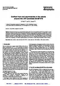
Fig. 1. Distribution of the [M/H] = 0 spectra incorporated in our stellar library (large symbols) in the log T eff − log g plane, compared to the position of stellar models of solar metallicity (small dots; these models are isochrones to be discussed later in Sect. 5.1). The spectra are taken from Castelli et al. (1997; crosses), Fluks et al. (1994; circles), Allard et al. (2000a; squares), and pure blackbody (triangles). Fluks et al. spectra have been arbitrarily located at log g = 0. Similar distributions hold for all metallicities between [M/H] = −2.5 and +0.5 (see text).

3. The stellar spectral library In the following, we will present the stellar spectral library put together for this work. For the sake of reference, Fig. 1 presents the distribution of all spectra in the log T eff − log g plane.

In the present work, we adopt the ATLAS9 no-overshoot models that have been calculated by Castelli et al. (1997). They correspond to the “NOVER” files available at http://cfaku5.harvard.edu/grids.html. The metallicities cover the values [M/H] = −2.5, −2.0, −1.5, −1.0, −0.5, 0.0, and +0.5, with solar-scaled abundance ratios. A microturbulent velocity ξ = 2 km s−1 , and a mixing length parameter α = 1.25, are adopted. Notice that these models are now being extended so as to include also α-enhanced chemical mixtures, which represents a potentially important improvement for our future works. Kurucz models cover quite well the region of the log T eff vs. log g plane actually occupied by stars, at least in the 3500 K ≤ T ≤ 50 000 K, 0 ≤ log g ≤ 5 intervals (see Fig. 1). However, it has to be extended to both lower and higher T eff s, as will be detailed below. It is important to recall that Kurucz (ATLAS9) spectra are widely used in the field of synthetic photometry, mainly because of their wide coverage of stellar parameters and easy availability. Moreover, there are also good indications in the literature that these spectra do a good job in synthetic photometry, provided that we are dealing with broad-band systems. Compelling examples of this can be found in Bessell et al. (1998), who compares the U BVRI JHKL results obtained from the recent ATLAS9 spectra to empirical relations derived with the infrared flux method, lunar occultations, interferometry, and eclipsing binaries. Their results indicate that the 1998 ATLAS9 models are well suited to synthetic photometry, but for small errors, generally lower than 0.1 mag in colours, that we do not consider as critical. In fact, we are more interested in the overall dependencies of colours and magnitudes with stellar parameters – probably well represented by present synthetic spectra – than on details of this order of magnitude. Additionally, Worthey (1994) presented extensive comparisons between Kurucz (1993) spectra and stars in the lowresolution spectral library by Gunn & Stryker (1983), obtaining generally a good match for wavelengths redder than the B passband. Worthey’s Fig. 9 also presents a comparison between Kurucz (1993) solar spectra and Neckel & Labs (1984) data, with excellent results (errors lower than 0.1 mag) all the way from the UV up to the near-IR. Since the ATLAS9 1998 spectra differ just little from the Kurucz (1993) version (a few percent in extreme cases), these results are to be considered still valid.

200


3.1.2. Some caveats on ATLAS9 spectra The previously mentioned works point to a reasonably good agreement between ATLAS9 spectra and those of real stars of near-solar metallicity, especially in the visual and near-infrared pass-bands. However, there are many known inadequacies in these spectra, which should be kept in mind as well. Here, we give just a brief list of the potential problems, concentrating on those which may be more affecting our synthetic colours. ATLAS9 spectra are based on 1D static and plan-parallel LTE model atmospheres, which use a huge database of atomic line data (Kurucz 1995). The line list is known not to be accurate: In fact, Bell et al. (1994) show that the solar spectra calculated using Kurucz list of atomic data present many unobserved lines; moreover, the number of lines which are too strong exceeds those which are too weak. The problem can be appreciated by looking at the high-resolution spectral plots presented by Bell et al. (1994), but could hardly be noticeable in low-resolution plots (such as in the comparisons presented in Worthey’s 1994 Fig. 9, and in Castelli et al. 1997 Fig. 2). Also, Bell et al. (2001) show that a motivated increase in the Fe  bound-free opacity cause a significant improvement in the fitting of the solar spectrum in the 3000–4000 Å wavelength region, affecting the entire UV region as well. Such increased sources of continuous opacity are still missing in ATLAS9 atmospheres2 . These results indicate that ATLAS9 spectra will produce worse results when applied to (i) narrow-band photometric systems, in which individual metallic lines can more significantly affect the colours, and (ii) in the UV region, especially shortward of 2720 Å (see Bell et al. 2001). In both cases, the errors caused by wrong atomica data are such that we can expect not only systematic and T eff -dependent offsets in synthetic colours, but also a somewhat wrong dependence on metallicity. Clearly, these points are worth being properly investigated by means of detailed spectral comparisons. Regarding the present work, the above-mentioned problems (i) critically determine the inadequacy of synthetic colours computed for the Strömgren system (Girardi et al., in preparation), and (ii) may possibly cause significant errors in our synthetic HST/WFPC2 UV colours. Other potential problems worth of mention are: – The deficiencies in 1D atmosphere models and in the mixing length description of convection, as compared to exploratory 3D model atmospheres (e.g. Asplund et al. 2000). They should affect mainly the intermediate-strong lines with significant non-thermal broadening and in stars cooler than ∼6000 K. The consequences of spatial and thermal inhomogeneities in the atmosphere of the Sun and Procyon have been investigated by Allende Prieto et al. (2001, 2002); – Inadequacies in the hydrogen line computations. Especially affected are high members of the Balmer series in GK stars – due to inhomogeneities in real atmospheres and 2 In the original Kurucz (1993) spectra, a modest reduction of the continuous UV flux results from the adopted “approximate overshooting” scheme.

inadequate treatment of hydrogen line broadening in cool stars (see Barklem et al. 2000a,b) – and the core of Balmer lines and the region around the Paschen discontinuity and longward in A stars (Colina et al. 1996). In synthetic photometry, these inadequacies are expected to slightly affect the U and B magnitudes for A-F stars, but to have a greater effect in Strömgren indices; – The inadequacy of using scaled-solar metal ratios in giants where the abundance of CNO elements has been altered by dredge-up events. Similarly, the inadequancy of using scaled-solar abundances for halo and bulge stars, instead of α-enhanced ones. Obviously, some improvement upon these points is expected in future releases of ATLAS spectra (see Castelli & Kurucz 2001), and of other extended spectral grids as well. Fortunately, the work by Bessell et al. (1998) gives us some confidence that present broad-band magnitudes and colours (from U to K) are modelled with an accuracy that is already acceptable for many applications. Finally, we remark that some authors (Lejeune et al. 1997, 1998) propose the application of a posteriori transformations to Kurucz (1993) spectra, as a function of wavelength and T eff , such as to reduce the errors of the derived synthetic U BVRI JHKL photometry. In our opinion, such transformations are questionable because they do not correct the cause of the discrepancies – majorly identifiable in the imperfect modelling of absorption lines – and the case for applying them to stars of all surface metallicities and gravities is far from compelling.

3.2. Extension to higher temperatures For T eff > 50 000 K, we simply assume black-body spectra. This is probably a good approximation for wavelengths λ > 912 Å. In fact, we find always a reasonably smooth transition in the computed BCS λ s as we cross the T eff = 50 000 K temperature boundary.

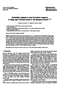
3.3. Extension to M giants Synthetic spectra for M giants have still many problems – mainly in their ultraviolet-blue region – that partially derive from incomplete opacity lists of molecules such as TiO, VO and H2 O (see e.g. Plez 1999; Alvarez & Plez 1998; Alvarez et al. 2000; and Houdashelt et al. 2000a,b to appreciate the state of the art in the field). Therefore, we prefer to use the empirical M giant spectra from Fluks et al. (1994; or “intrinsic” spectra as referred in their paper). They cover the wavelength interval from 3800 Å to 9000 Å. Outside this interval, the empirical spectra have been extendend with the “best fit” synthetic spectra computed by the same authors. However, the whole procedure reveals a problem: if we simply merge empirical and synthetic spectra from Fluks et al. (1994), the resulting synthetic B−V and U −B colours just badly correlate with the measured colours for the same stars (which were also obtained by Fluks et al. 1994). This problem


probably derives from a bad flux calibration at the blue extremity of the observed spectra and/or from the imperfect match between synthetic and observed spectra at 3800 Å. In order to circumvent (at least partially) the problem, we simply multiply each M-giant spectrum blueward of 4000 Å (with a smooth transition in the range from 4000 Å to 4800 Å) by a constant, typically between 0.8 and 1.2, so that the synthetic colours recover the observed behaviour of the B−V vs. V −K data. The first two panels of Fig. 2 show the results. Actually, Fig. 2 presents six different colour vs. V −K diagrams that are useful to understand the situation for giants. Care has been taken in expressing data and models in the same photometric system, the “Bessell” U BVRI JHK one, that we will detail later in Sect. 4.1. For M giants, the empirical photometric data from Fluks et al. (1994; small dots) can be compared with the results of our synthetic photometry 3. Noteworthy, there is a reasonably good match between the synthetic and observed relations for most colours. This has been imposed for U −B and B−V, whereas is a natural result for all colours involving wavelengths longer than ∼4800 Å. The only clear exception is the V −R colour, for which differences of ∼0.4 mag are found for all giants of spectral type later than M4 (V −K > ∼ 5). The reason for this discrepancy is not clear, but may lie in the use of R filters with different transmission curves. Also the predictions for J −K do not fit well all the photometric data, somewhat failing for the spectral types later than M7 (V −K > ∼ 8). However, since these latters are quite rare, such mismatch does not pose a serious problem. For the sake of comparison, Fig. 2 also presents the relations obtained by means of the M-giant models from Houdashelt et al. (2000a), in the case of solar metallicity. Together with other recent examples (e.g. Plez 1999; Alvarez et al. 2000), they represent state-of-the-art computations of cool oxygen-rich stellar atmospheres. As can be appreciated in the figure, Houdashelt et al. models reproduce well the empirical data as far as V −K < ∼ 6 (spectral types earlier than M5), but start departing from these for cooler stars. A similar situation holds if we look at different T eff –colour relations, as can be seen in Figs. 13 and 14 of Houdashelt et al. (2000a), where they compare their T eff –colour relations with those obtained with Fluks et al. (1994) spectra and data for field giants. Also in this case, it seems that Fluks et al. (1994) spectra do better reproduce the empirical relations for the spectral types later than M4. Once we have defined the library of M-giant spectra, we associate effective temperatures to them by using the scale favoured by Fluks et al. (1994). In this scale, M giants cover the temperature interval from 3 850 K (MK type M0) to 2500 K (MK type M10). We recall that Fluks et al. (1994) T eff values are derived from a careful fitting of the observed spectra with synthetic model atmospheres of solar metallicity. Their scale is also in excellent agreement with the empirical one from Ridgway et al. (1980), which covers spectral types earlier than M6. 3 The JHK colours from Fluks et al. are in the ESO system and have been converted to the Bessell one by using the relations found in Bessell & Brett (1988).

201

After the proper T eff is attributed, each one of our modified spectra is completely re-scaled by a constant, so that the total 4 – is recovered. flux vs. T eff relation – i.e. Fbol = σT eff Finally, we face the problem of defining the transition between the M-giant spectra, and the ATLAS9 ones which are available for temperatures higher than 3500 K. To this aim, it is helpful to examine Fig. 2, where we also include: – the synthetic photometry for a sequence of ATLAS9 spectra for M giants (empty circles). These spectra are located along the line T eff = 3250 + 500 log g, which represents fairly well the locus of low-mass red giants in a T eff vs. log g diagram (see Fig. 1); – the mean empirical relations for F0–K5 giants of [Fe/H] = 0 as derived from Alonso et al. (1999b) fitting formulas (dashed lines)4 . An important fact to be noticed is that our synthetic photometry reproduces Alonso et al. (1999b) relations in all colours remarkably well. From inspecting this and other similar plots, we can conclude that the mismatch between Kurucz ATLAS9 and Fluks et al. (1994) spectra starts at about T eff = 3850 and increases slowly as the temperature decreases down to 3500 K (i.e. from V −K ' 3.5 to V −K ' 4.7). Hence, we adopt a smooth transition between these two spectral sources over this temperature interval. The same M giant spectra are assumed for all metallicities. The complete procedure ensures reasonable colour vs. V −K relations for all giants of near-solar metallicity (Fig. 2). Nevertheless, this kind of approach cannot be completely satisfactory, first because the original Fluks et al. (1994) spectra have been artificially corrected at wavelengths shorter than 4800 Å in order to produce reasonable B−V and U −B, and second because we do not dispose of similar M-giant spectra for metallicities very different from solar. Better empirical and theoretical spectra for M giants seem to be urgently needed. Anyway, in the context of the present work the problem is not dramatic because M giants cooler than T eff ∼ 3500 K are only found in the RGB-tip and TP-AGB phases of high metallicity stellar populations, and constitute just a tiny fraction of the number of red giants. The problem could be critical, instead, when we consider integrated properties of stellar populations, because M giants, despite their small numbers, have high luminosities and contribute a sizeable fraction of the integrated light.

3.4. Extension to M+L+T dwarfs Although the modelling of cool dwarfs atmospheres presents challenges comparable to those found in late-M giants (e.g. the inadequacy of TiO and H2 O line lists, and dust formation; see Tsuji et al. 1996, 1999; Leggett et al. 2000), present results Alonso et al. (1999b) V −I and V −R colours have been transformed from Johnson to Johnson-Cousins systems using relations from Bessell (1979), whereas infrared colours were converted from TCS to “Bessell” systems using the relations from Alonso et al. (1998). 4

202


Fig. 2. Colour vs. V −K relations for giants. The connected open circles represent the relation obtained from [M/H] = 0 ATLAS9 spectra located along the T eff = 3250 + 500 log g line (the typical location for RGB stars) in the diagram of Fig. 1. The connected open squares correspond to the relation obtained from the M-giant spectra from Fluks et al. (1994), completed and modified at λ < 4800 Å as detailed in the text. The dashed lines represent the empirical relations for F0–K5 solar-metallicity giants from Alonso et al. (1999b), whereas the dotted lines are the synthetic relations for K0–M7 giants from Houdashelt et al. (2000a). The empirical data for M giants (small dots) are from Fluks et al. (1994). As far as possible, all observations have been converted to the same photometric system as used in our synthetic photometry (i.e. the “Bessell” U BVRI JHK system; see text).

compare reasonably well with observational spectral data (see e.g. Fig. 9 in both Leggett et al. 2000 and 2001). A review on the subject can be found in Allard et al. (1997). An extended library of synthetic spectra for cool dwarfs (of types M and later) is provided by Allard et al. (2000a; see ftp://ftp.ens-Lyon.fr/pub/users/CRAL/fallard). We use their set of “BDdusty1999” atmospheres (see also Chabrier et al. 2000; Allard et al. 2000b, 2001), that should supersede the “NextGen” models from the same group

(Hauschildt et al. 1999) due to the consideration of better opacity lists and dust formation. Dust can significantly affect the coolest atmospheres, corresponding to dwarfs of spectral types L and T. The selected spectra cover the T eff intervals: – from 4000 K to 2800 K (“AMES” models) for metallicities [M/H] = 0.0, −0.5, −1.0, −1.5, and both log g = 5.0 and 5.5;


– from 2800 K down to 500 K (“AMES-dusty” models) only for [M/H] = 0.0, and log g values between 3.5 and 6.0. These spectra are presented with a extremely high resolution, that by far exceeds the one necessary in our work. Thus, we have convolved the flux per unit frequency Fν with a Gaussian filter of σν = 2.4 × 10−18 Hz, that corresponds to a FWHM of 20 Å at λ = 5550 Å. The resulting spectra were then reported to the same grid of wavelengths of Kurucz’ spectra. We find that there is a good agreement between ATLAS9 and BDdusty1999 spectra in the T eff range between ∼3800 K and 4000 K. Then, we set the transition between ATLAS9 and BDdusty1999 spectra at ∼3900 K. This choice guarantees smooth T eff vs. colour relations for dwarfs.

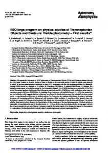
4. Photometric systems available In this section we present the basic information regarding the filter transmission curves and zero-points for each photometric system. As a reference to the discussion, Fig. 3 presents the filter sets under consideration, as compared to the spectra of a hot (Vega), an intermediate (the Sun), and a cool star (an M5 giant).

4.1. Johnson-Cousins-Glass system Aiming to reproduce the Johnson-Cousins-Glass system, we adopt the filter pass-bands indicated by Bessell (1990; for Johnson-Cousins U BVRI) and Bessell & Brett (1988; for JHK). We also apply their prescription for computing the U −B colour by means of a slightly modified pass-band BX90 , instead of the normal B one. Moreover, in order to better recover the original system, we adopt energy instead of photon count integrations (see Sect. 2.1). It is worth recalling that these pass-bands represent just one specific version of the “standard” Johnson-Cousins-Glass system, that may differ from filter systems in usage at several observatories. The Bessell & Brett (1988) JHKLM pass-bands, for instance, represent an effort in the direction of homogenizing several different near-infrared systems (SAAO, ESO, CIT/CTIO, MSO, AAO, and Arizona). In Bessell (1990) and Bessell & Brett (1988), the reader can find a set of useful fitting relations between colours in the several original systems. As previously mentioned, Johnson-Cousins-Glass is essentially a VEGAmag system. We fix the zero-points by assuming that Vega has apparent magnitudes equal to 0.03 in all U BVRI JHK bands, i.e. we impose all colours to be null. Notice that our definition is very similar to the Bessell et al. (1998) one, who adopt Vega colours differing from zero by just some thousandths of a magnitude (see their Table A1).

203

4.2.1. WFPC2 As for the WFPC2, we produce bolometric corrections and magnitudes in the F170W, F218W, F255W, F300W, F336W, F439W, F450W, F555W, F606W, F702W, F814W, and F850LP filters. Similar tables have been produced in previous papers (Chiosi et al. 1997; Salasnich et al. 2000); the present ones differ just in minor details. The transformations have been computed in STmag, ABmag, and VEGAmag systems. Whereas the STmag and ABmag systems can be straightforwardly simulated, the VEGAmag one deserves some comments. According to the SYNPHOT package distributed with the STSDAS software, in a VEGAmag system Vega should have apparent magnitudes equal to zero in all pass-bands. However, the most widely used calibration of WFPC2 photometry comes from Holtzman et al. (1995), who adopt a set of zero-points in which Vega has apparent magnitudes U = 0.02, B = 0.02, V = 0.03, R = 0.039, I = 0.035. Accordingly, we choose this latter definition, and impose that for the WFPC2 filters that correspond to U BVRI in wavelength, the synthetic magnitudes of Vega have these same values. For filters of intermediate wavelength, we adopt a linear interpolation between these values, whereas for bluer and redder filters a Vega magnitude equal to zero is assumed. As for the S λ functions, we use the pre-launch pass-bands kindly provided by Jon Holtzman (see Holtzman et al. 1995). We recall that, owing to the presence of contaminants inside the WFPC2 (see Baggett & Gonzaga 1998; Holtzman et al. 1995), S λ changes slowly with time, especially for UV filters. To cope with this, observers usually apply small corrections to the definition of the instrumental magnitudes, in order to bring the magnitudes back to the original conditions (see Holtzman et al. 1995). This justifies our use of pre-launch pass-bands instead of the present-day ones provided by SYNPHOT.

4.2.2. NICMOS For NICMOS filters, we compute bolometric corrections and absolute magnitudes in the ABmag, STmag, and VEGAmag systems. For the moment, calculations are limited to the three most frequently used filters, i.e. F110W, F160W, and F205W. The pass-bands come from SYNPHOT, and have been kindly provided by Don Figer. NICMOS observations are also frequently expressed in units of milli-Jansky (mJy). The conversion between AB magnitudes and mJy is straightforward: mAB,ν (mag) = −2.5 log fν (mJy) − 16.4.

(16)

4.2. Instruments on board of HST

4.3. ESO Imaging Survey (EIS) filter sets

In the context of the present work, the distinctive feature of HST photometry is the use of ABmag and STmag systems, which greatly simplifies the definition of zero-points. WFPC2 and NICMOS observations can also be expressed in VEGAmag magnitudes.

The EIS survey (Renzini & da Costa 1997; da Costa 2000) aims at providing a large database of deep photometric data, among which the astronomical community could select interesting targets for VLT spectroscopy. The survey is conducted at several different instruments at ESO.

204


Fig. 3. The filter sets used in the present work. From top to bottom, we show the filter+detector transmission curves S λ for the systems: (1) HST/NICMOS, (2) HST/WFPC2, (3) Washington, (4) ESO/EMMI, (5) ESO/WFI U BVRIZ + ESO/SOFI JHK, and (6) Johnson-CousinsGlass. All references are given in Sect. 4. To allow a good visualisation of the filter curves, they have been re-normalized to their maximum value of S λ . For the sake of comparison, the bottom panel presents the spectra of Vega (A0V), the Sun (G2V), and a M5 giant, in arbitrary scales of Fλ .

4.3.1. WFI The Wide Field Imager (WFI) at the MPG/ESO 2.2 m La Silla telescope provides imaging of excellent quality over a 340 × 330 field of view. It contains a peculiar set of broad-band filters, very different from the “standard” Johnson-Cousins ones. This can be appreciated in Fig. 3; notice in particular the particular shapes of the WFI B and I filters. Moreover, EIS makes use of the WFI Z filter which does not have a correspondency in the Johnson-Cousins system. Given the very unusual set of filters, the importance of computing isochrones specific for WFI is evident. This has benn done so for the broad WFI filters U (ESO#841), B (ESO#842),

V (ESO#843), R (ESO#844), I (ESO#845), and Z (ESO#846), that – here and in Fig. 3 – are referred to as U BVRIZ for short. Bolometric corrections have been computed in the VEGAmag system assuming all Vega apparent magnitudes to be 0.03, and in the ABmag system, which is adopted by the EIS group. The photometric calibration of EIS data is discussed in Arnouts et al. (2001). It is very important to notice that any photometric observation performed with WFI that makes use of standard stars (e.g. Landolt 1992) to convert WFI instrumental magnitudes to the standard Johnson-Cousins U BVRI system, will not be in the WFI VEGAmag system we are dealing with here. Instead, in


that case, we should better compare the observations with the isochrones in the standard Johnson-Cousins system, or, alternatively, apply colour transformations to our WFI isochrones so that they reproduce the T eff -colour sequences of dwarfs and giants in the Johnson-Cousins system. This aspect will be better illustrated Sect. 6.

205

Since the procedure for computing BCS λ tables is relatively easy, provided the necessary information – i.e. filter transmission curves and a zero-point definition that corresponds to one of the cases discussed in Sect. 2.3 – is given, we can provide isochrone tables for any photometric systems upon request.

5. Available stellar tracks and isochrones 4.3.2. SOFI SOFI is a near-infrared imager and grism spectrograph at the ESO NTT 3.6 m telescope. It is used to complement WFI observations in near-infrared pass-bands. More specifically, it disposes of J, H and Ks filters that have some similarity to Glass JHK (see Fig. 3). VEGAmag magnitudes are computed assuming the same as before, i.e. that Vega apparent magnitudes are 0.03.

4.3.3. EMMI EMMI is a visual imager and grism spectrograph also at the NTT. The EIS project uses a set of its wide filters, i.e. Bw , Iw , Rw , and Vw , together with the R filter. The pass-bands have been kindly provided by S. Arnouts. As before, VEGAmag magnitudes are computed assuming that Vega has 0.03 mag in all filters.

4.4. Washington system The Washington system, originally defined by G. Wallerstein and developed by Canterna (1976), has been more and more used since Geisler (1996) defined a set of CCD standard fields. In the present paper, we reproduce the Washington CCD system (filters C, M, T 1 and T 2 ) by adopting the transmission curves as revised by Bessell (2001). Following Geisler (1996), the Washington T 1 filter has been frequently replaced by the Kron-Cousins filter R, which presents a similar transmission curve and is available in almost all observatories. Additionally, Holtzman et al. (in preparation) suggest the use of BVI colours together with Washington ones for breaking the age-metallicity degeneracy of stellar populations in colour-colour diagrams. For these reasons, in all tables that deal with the Washington CMT 1 T 2 system, we also insert the information for the Johnson-Cousins BVRI filters. Finally, following Geisler (private communication), the zero-points should be well represented by a VEGAmag system. We assume Vega has magnitude 0.03 in all filters.

4.5. Other planned systems Forthcoming papers of this series will be dedicated to – other traditional systems like Strömgren, Thuan-Gunn, Vilnius, etc.; – systems corresponding to some successful and recent/ongoing observational campaigns, like Hipparcos, MACHO, DENIS, 2MASS, and SDSS; – newly-proposed systems, like the ones for the future astrometric mission GAIA.

The tables of bolometric corrections here described have been primarily constructed to be applied to the Padova database of stellar evolutionary tracks and isochrones5. These latter have been described in several previous papers, and a complete description of them is beyond the scope of this work. In the following, our intention is just to briefly mention the sets of isochrones which are the most useful for comparisons with observed photometric data, and to first mention some data that has not been published in precedence. A summary table of the available material is presented in Table 1.

5.1. An extended set of isochrones Girardi et al. (2000) computed a set of low- and intermediatemass stellar tracks which supersedes those previously used in Bertelli et al. (1994) isochrones. Additional models (unpublished) have been recently computed for initial chemical composition [Z = 0.0001, Y = 0.23]. Thus, we have created a new set of isochrones combining the latest low- and intermediate mass tracks (in the range 0.15−7.0 M ) with the formerly available massive ones. The full references are given in Table 1. In all cases in which “2000” and “1994” tracks have been combined, we find excellent agreement between the relevant quantities (lifetimes, tracks in the HR diagram) at the transition mass of 7−8 M . This is explained considering that the intermediate- and high-mass models share the same prescription for convection, and have interior opacities dominated by electron scattering (which has not been changed in the meanwhile). For the solar metallicity, we have combined tracks presenting slightly different initial metallicities – [Z = 0.019, Y = 0.273] in Girardi et al. (2000), and [Z = 0.020, Y = 0.280] in Bressan et al. (1993) – without finding any significant discontinuity. Finally, to this extended set we have included the Marigo et al. (2001) isochrones for zero-metallicity stars.

5.2. Overshooting vs. classic models For solar metallicity and in the mass range 0.15−7.0 M , Girardi et al. (2000) presents an additional set of tracks and isochrones computed with the classical semi-convective prescription for convective borders. Then, the two [Z = 0.019, Y = 0.273] sets are useful if one chooses to compare classical with overshooting models. The same kind of work is being extended to metallicities [Z = 0.004, Y = 0.240] and [Z = 0.008, Y = 0.250] (Barmina et al. 2002), and will be included in the database when completed. 5

Of course, they can also be applied to any other set of stellar data in the literature.

206


Table 1. Stellar tracks used in the different set of isochrones. Initial chemical comp.:

Evolutionary tracks:

Z

Y

kind1

Mass ranges (in M ): 0.15–0.55 0.6–7.0

0.0 0.0001 0.0004 0.001 0.004 0.008 0.019 0.030

0.230 0.230 0.230 0.230 0.240 0.250 0.273 0.300

S S S S S S S S

– Gi01 Gi00 Gi00 Gi00 Gi00 Gi00 Gi00

0.019

0.273

S

0.008 0.019 0.040 0.070 0.008 0.019 0.040 0.070

0.250 0.273 0.320 0.390 0.250 0.273 0.320 0.390

0.004 0.008 0.019

0.240 0.250 0.273

Isochrones: 2

>7.0

TP-AGB evolution3

convection4

age range log(t/yr)

filename in database

basic reference2

Ma01 Gi01 Gi00 Gi00 Gi00 Gi00 Gi00 Gi00

Ma01 Gi96 Fa94a – Fa94b Fa94b Br93 –

– G G G G G G G

O O O O O O O O

6.30−10.25 6.60−10.25 6.60−10.25 7.80−10.25 6.60−10.25 6.60−10.25 6.60−10.25 7.80−10.25

isoc isoc isoc isoc isoc isoc isoc isoc

Ma01 Gi01+Gi96 Gi00+Be94 Gi00 Gi00+Be94 Gi00+Be94 Gi00+Be94 Gi00

Gi00

Gi00

–

G

C

7.80−10.25

isoc z019nov.dat

Gi00

S S S S A A A A

Sa00 Sa00 Sa00 Sa00 Sa00 Sa00 Sa00 Sa00



G G G G G G G G

O O O O O O O O

7.00−10.25 7.00−10.25 7.00−10.25 7.00−10.25 7.00−10.25 7.00−10.25 7.00−10.25 7.00−10.25

isoc isoc isoc isoc isoc isoc isoc isoc


S S S

Gi00 Gi00 Gi00

Gi00 Gi00 Gi00

– – –

M M M

O O O

7.80−10.25 7.80−10.25 7.80−10.25

isoc z004m.dat isoc z008m.dat isoc z019m.dat

z0.dat z0001.dat z0004.dat z001.dat z004.dat z008.dat z019.dat z030.dat

z008s.dat z019s.dat z040s.dat z070s.dat z008a.dat z019a.dat z040a.dat z070a.dat

MG01 MG01 MG01

S indicates a solar-scaled distribution of metals, A indicates an α-enhanced one. The adopted metal abundance ratios are specified in Salasnich et al. (2000). 2 References for tracks and isochrones: Be94 = Bertelli et al. (1994, A&AS, 106, 275); Br93 = Bressan et al. (1993, A&AS, 100, 647); Fa94a = Fagotto et al. (1994a, A&AS, 104, 365); Fa94b = Fagotto et al. (1994b, A&AS, 105, 29); Gi96 = Girardi et al. (1996, A&AS, 117, 113); Gi00 = Girardi et al. (2000, A&AS, 141, 371); Gi01 = Girardi (2001, unpublished); Ma01 = Marigo et al. (2001, A&A, 371, 152); MG01 = Marigo & Girardi (2001, A&A, 377, 132); Sa00 = Salasnich et al. (2000, A&A, 361, 1023). 3 G means a simple synthetic evolution as in Girardi & Bertelli (1998), whereas M stands for more detailed calculations as in Marigo (2001; and references therein). 4 O means a model with overshooting (see Gi00 for all references), whereas C corresponds to classical semi-convective models. 1

5.3. Solar-scaled vs. α-enhanced models Salasnich et al. (2000) presents new models for 4 different metallicities ([Y = 0.250, Z = 0.008], [Y = 0.273, Z = 0.019], [Y = 0.320, Z = 0.040] and [Y = 0.390, Z = 0.070]), computed both with scaled-solar and alpha-enhanced distributions of metals. The tracks cover the mass range from 0.15 to 20 M . They represent a valid alternative to the isochrones referred to in Sect. 5.1, but do not cover the low-metallicity interval. Anyway, it has been demonstrated by Salaris et al. (1993; see also Salaris & Weiss 1998; and VandenBerg 2000), that for low metallicities one may safely use scaled-solar stellar models instead of α-enhanced ones of same Z.

5.4. Simple vs. more detailed TP-AGB models All the tracks and isochrone sets above mentioned, include the complete TP-AGB phase as computed with a simple synthetic algorithm (Girardi & Bertelli 1998). In parallel, Marigo (2001, and references therein) has developed a much more sophisticated code for synthetic TP-AGB evolution, which includes crucial processes such as the third dredge-up and

hot-bottom burning. Sets of complete TP-AGB tracks have been so far presented for metallicities [Y = 0.240, Z = 0.004], [Y = 0.250, Z = 0.008], and [Y = 0.273, Z = 0.019] (Marigo 2001). A set of isochrones has been generated by combining these detailed TP-AGB tracks with the previous evolution from Girardi et al. (2000); they are presented in the appendix of Marigo & Girardi (2001). These isochrones represent a useful alternative to the isochrones referred to in Sect. 5.1, any time the TP-AGB population is under scrutiny – for instance, when we have nearinfrared photometry of objects above the RGB-tip. Marigo TPAGB models are being extended to cover a larger metallicity interval.

6. Discussion and concluding remarks

6.1. Summary This work is dedicated to the presentation of theoretical isochrones in several photometric systems. It represents the continuation of a wide project of the Padova group, started with Bertelli et al. (1994) and then carried on by Chiosi et al. (1997),


and more recently by Salasnich et al. (2000). It starts describing the formalism for converting synthetic stellar spectra into tables of bolometric corrections (Sect. 2), in such a way that it can be easily applied to different photometric systems, and with the possibility of including extinction in a self-consistent way. Then, we describe the assemblage of an updated library of stellar spectra (Sect. 3). The library is quite extended in T eff and log g, and includes the crucial dependence of spectral features on metallicity. Of course, it suffers from some limitations: very hot stars and M-giants are not included among synthetic spectra, a situation which can be remediated by using blackbody and empirical spectra, respectively. The strinkingly different spectra of carbon stars will also have to be considered in the future (Marigo et al., in preparation). These are probably the points where the models can be most improved. Moreover, several problems may be affecting the ATLAS9 synthetic spectra we are using to simulate the broad-band colours of most stars (see Sect. 3.1). Although such spectra have been demonstrated to be suitable for synthetic photometry (mainly for the Johnson-Cousins-Glass system; e.g. Bessell et al. 1998), their accuracy has still to be sistematically evaluated for stars of all metallicities, temperatures and gravities. Anyway, we assume that they are good enough for simulating broad-band photometric systems in the visual-infrared wavelength region, whereas expect that the results in narrow-band systems, and in the ultraviolet pass-bands, will be affected by more significant errors. Another important aspect of synthetic spectra is that they are usually computed for scaled-solar chemical compositions, whereas the extension to peculiar and α-enhanced mixtures would be of high interest. This latter problem will probably be alleviated in a near future, with the release of extensions to ATLAS9 spectra. From the spectral library, we derive bolometric corrections for each pass-band mentioned in Sect. 4, and apply them to the Padova isochrones. In practice, only in few cases we present newly-constructed isochrones: the bulk of isochrone data is already described in previous papers by our group, and it is only the transformation from theoretical quantities to absolute magnitudes that changes compared to past releases. Section 5 summarizes the basic characteristics of the different sets of isochrones, indicating the full references.

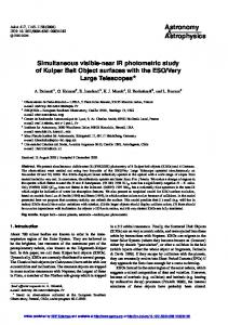
6.2. Comparison with previous works It is important to illustrate the differences between the present and previous transformations. The previous ones for U BVRI JHK are fully described in Bertelli et al. (1994), and were adopted by Girardi et al. (2000), Salasnich et al. (2000) and Marigo et al. (2001); for HST/WFPC2 photometry, they are the ones described in Salasnich et al. (2000). The situation for Johnson-Cousins-Glass is tentatively illustrated in Fig. 4, which compares a set of Girardi et al. (2000) isochrones, transformed according to both present (continuous

207

lines) and Bertelli et al. (1994; dashed lines) transformations. We point out that: 1. For stars hotter than T eff ∼ 4000 K, present transformations are very similar to those of Bertelli et al. (1994). The differences amount to just a few hundredths of a magnitude over most regions of the CMD, including the entire main sequence and subgiant branch, and most of the RGB. They can be entirely attributed to the slightly different pass-bands and zero-points, and to the use of more recent ATLAS9 “NOVER” atmospheres instead of Kurucz (1993) ones; 2. A somewhat similar situation holds for dwarfs cooler than T eff ∼ 4000 K (see bottom end of the main sequence in all panels, for MV > ∼ 7, and MK > ∼ 5). The differences are generally small and can be attributed to the change from Kurucz (1993) to Allard et al. (2000a) spectra. The exceptions are U −B and J −H colours, for which the differences between the two versions become sizeable; 3. For giants cooler than 4000 K, present transformations become very different. This can be noticed in the upperright corner of all diagrams. M-giants corresponding to the RGB-tip and TP-AGB, are now seen to fade by some magnitudes in V, due to a sort of rapid increase of visual BCs at T eff < ∼ 3500 K. This effect is caused by the use of Fluks et al. (1994) spectra and their T eff vs. V −K scale. Such a bending of the RGB is indeed observed in CMDs of old metal-rich clusters (see e.g. Ortolani et al. 1990; and Rich et al. 1998), and seems to be better reproduced now than with previous transformations. Other differences appear in all colours: the most remarkable are the excursion of M-giants of latest type towards much bluer U −B, and the much smoother behaviour now obtained for J −H and H−K. A quite similar situation holds for HST/WFPC2 photometry, as illustrated in Fig. 5. This time, we compare the same isochrones as transformed with present (continuous lines) and Salasnich et al. (2000; dashed lines) transformations. It is evident that the present transformations ensure a more continuous behaviour of the colours for all low-temperature stars (both dwarfs and giants). From the plots at the top row of Fig. 5, one can also appreciate the unusual appearance of isochrones in CMDs that involve ultraviolet WFPC2 pass-bands: Notice for instance that in F170W, F218W, F255W and F330W magnitudes, giants may be fainter than turn-off stars. Isochrones in the F218W vs. F170W−F218W and F255W vs. F218W−F255W diagrams are even “twisted”, because the T eff vs. colour relations are not monotonic for these filters. These effects are related to the presence of a red leak in the ultraviolet HST filters (for both the present WFPC2 and the former FOC camera), and are extensively discussed by Yi et al. (1995) and Chiosi et al. (1997). As a consequence of the great similarity between present and previous U BVRI JHK and HST/WFPC2 transformations, for most colours and over a large portion of the HR diagram, most results derived from previous Padova isochrones are not expected to change. Exceptions may show up for works that are concerned with the photometry of the reddest giants, with T eff < ∼ 3500 K (B−V > ∼ 1.5), or that deal with low-mass mainsequence stars in the U −B and ultraviolet colours.

208


Fig. 4. Comparison of Girardi et al. (2000) isochrones transformed to Johnson-Cousins-Glass magnitudes and colours by using either present relations (continuous lines) or Bertelli et al. (1994) ones (dashed lines), in several CMDs. The isochrones have solar metallicity (Z = 0.019) and ages 108 , 109 , and 1010 yr (from top to bottom).

6.3. New results The greatest improvement of the present database is in the presentation of Padova isochrones in several photometric systems for which they were not available so far – including the case of brand-new systems. Three examples of theis kind are given in Figs. 6–8. First, Fig. 6 presents the isochrones in NICMOS ABmag system. In a VEGAmag system, NICMOS isochrones would look similar to their equivalent Johnson-Cousins-Glass ones, shown in Fig. 4. In the ABmag system, however, they appear shifted to quite different colour and magnitude intervals.

Figure 7 illustrates how Padova isochrones look like in the T 1 vs. C − T 1 CMD of Washington photometry, both for varying age at constant metallicity (left panel), and for varying metallicity at constant age (right one). The striking feature in these plots is the excellent separation in metallicity offered by the C − T 1 colour, from the main sequence up to red giant phases. This feature, combined to the excellent throughput in the C filter (Fig. 3), is among the advantages that make the Washington system a very competitive one if compared to Johnson-Cousins (see also Paltoglou & Bell 1994; Geisler & Sarajedini 1999).


209

Fig. 5. Comparison of Girardi et al. (2000) isochrones as transformed to the WFPC2 VEGAmag system using either present relations (continuous lines) or Salasnich et al. (2000) ones (dashed lines). The isochrone ages and metallicities are the same as in Fig. 4.

Preliminary comparisons point to a good agreement between our Washington isochrones and real data for LMC fields from Bica et al. (1998). Just to mention an example, we notice that C − T 1 for giants “saturates” at ∼3.4, both in the models and in the LMC data. An example of “new” photometric system is provided by the WFI, which has broad-band filters very different from Johnson-Cousins ones. To illustrate the effect in colours, Fig. 8 shows exactly the same isochrones as seen in BVI CMDs using either Johnson-Cousins or WFI filters, and applying in both cases the VEGAmag definition of zero-points. The differences are striking. In particular, since the BV WFI filters represent a wavelength baseline shorter than the Johnson ones, they

provide a more modest separation of stars in B−V colour. It is evident from this plot that the normal Johnson-Cousins isochrones cannot be used to interpret WFI data that has been converted to VEGAmag or ABmag systems, as for most of EIS data (e.g. Arnouts et al. 2001; Groenewegen et al. 2002)6 .

6.4. Retrieval of electronic tables All the data here mentioned are available at the WWW site http://pleiadi.pd.astro.it. The database already 6 Notice, however, that part of the data released from EIS – namely the pre-FLAMES survey – is in fact converted into a standard Johnson-Cousins system (see Momany et al. 1901).

210


Fig. 6. Isochrones in the CMDs of NICMOS ABmag photometry. Ages and metallicities are the same as in Fig. 4.

Fig. 7. Isochrones in the T 1 vs. C − T 1 plane of Washington photometry. Left panel: from top to bottom, a sequence of Z = 0.008 isochrones with ages 107 , 108 , 109 , and 1010 yr. Right panel: from left to right, a sequence of 14 Gyr old isochrones with metallicities Z = 0.0001, 0.0004, 0.001, 0.004, 0.008, 0.019, and 0.030.

includes a very large number of files, and is expected to increase further as we publish data for other photometric systems. Thus, it is hard to describe here both the structure of the database, and the content of each file. Moreover, this kind of information is probably useful just to whom actually accesses the database. Thus, we opt to provide all the relevant information in readme.txt files inserted in the database. To the general reader, suffice it to briefly mention the kind of data which is available: – Tables of bolometric corrections for each metallicity: they contain the quantities BCS λ for each filter, and as a function of stellar T eff and log g. Metallicities available are [Fe/H] = −2.0, −1.5, −1.0, −0.5, 0, +0.5. The values of T eff and log g

are not exactly the same for all metallicities, but correspond quite well to the regions indicated in Fig. 1; – Tables of isochrones: they include all metallicities and cases indicated in Sect. 5. The various photometric systems are separated in different directories. For each isochrone file, the information and structure are the same as already presented in Girardi et al. (2000), Salasnich et al. (2000), and Marigo & Girardi (2001), with the obvious difference that instead of U BVRI JHK absolute magnitudes, in each file we tabulate the absolute magnitudes for the photometric system under consideration; – Tables of integrated colours of single-burst stellar populations: a table of this kind is present for each isochrone table. They provide integrated magnitudes in each pass-band, as a function of age.


211

Fig. 8. Comparison between the same set of Z = 0.019 isochrones as seen in the U BV I CMDs using either Johnson-Cousins (dashed lines) or WFI filters (continuous lines). VEGAmag systems are used in both cases. Ages are the same as in Fig. 4. Acknowledgements. L.G. thanks the many people who helped by providing filter transmission curves and zero-points information (in particular E. Bica, D. Geisler, J. Holtzman, D. Figer, E. Grebel, M. Gregg, M. Rich, S. Arnouts, and L. da Costa). Particularly appreciated are the availability (R. Kurucz, F. Allard) and help with (I. Baraffe) online spectral data, the useful comments by B. Plez regarding cool giants, and the many useful remarks by R. Bell and M.S. Bessell, which greatly helped to improve this paper. Also acknowledged are those who kindly pointed out some mistakes in our preliminar releases of data. L.G. acknowledges a stay at MPA funded by the European TMR grant ERBFMRXCT 960086. This work was partially funded by the Italian MURST.

References Allard, F., Hauschildt, P. H., Alexander, D. R., & Starrfield, S. 1997, ARA&A, 35, 137 Allard, F., Hauschildt, P. H., Alexander, D. R., Tamanai, A., & Ferguson, J. W. 2000a, in Proc. of From giant planets to cool stars, ed. C. A. Griffith, & M. S. Marley, ASP Conf. Ser., 212, 127 Allard, F., Hauschildt, P. H., & Schwenke, D. 2000b, ApJ, 540, 1005 Allard, F., Hauschildt, P. H., Alexander, D. R., Tamanai, A., & Schweitzer, A. 2001, ApJ, 556, 357 Allende Prieto, C., Barklem, P. S., Asplund, M., & Ruiz Cobo, B. 2001, ApJ, 558, 830 Allende Prieto, C., Asplund, M., Garcia López, R. J., & Lambert, D. L. 2002, ApJ, 567, 544 Alonso, A., Arribas, S., & Mart´ınez-Roger, C. 1998, A&AS, 131, 209 Alonso, A., Arribas, S., & Mart´ınez-Roger, C. 1999a, A&AS, 139, 335 Alonso, A., Arribas, S., & Mart´ınez-Roger, C. 1999b, A&AS, 140, 261 Alvarez, R., Lan¸con, A., Plez, B., & Wood, P. R. 2000, A&A, 353, 322 Alvarez, R., & Plez, B. 1998, A&A, 330, 1109 Arnouts, S., Vandame, B., Benoist, C., et al. 2001, A&A, 379, 740 Asplund, M., Ludwig, H.-G., Nordlund, A., & Stein, R. F. 2000, A&A, 359, 669

Baggett, S., & Gonzaga, S. 1998, ISR WFPC2 98-03 Bahcall, J. N., Pinsonneault, M. H., & Wasserburg, G. J. 1995, Rev. Mod. Phys., 67(4), 781 Barklem, P. S., Piskunov, N., & O’Mara, B. 2000a, A&A, 355, 5 Barklem, P. S., Piskunov, N., & O’Mara, B. 2000b, A&A, 363, 1091 Barmina, R., Girardi, L., & Chiosi, C. 2002, A&A, 385, 847 Bell, R. A., Paltoglou, G., & Tripicco, M. J. 1994, MNRAS, 268, 771 Bell, R. A., Balachandran, S. C., & Bautista, M. 2001, ApJ, 546, L65 Bertelli, G., Bressan, A., Chiosi, C., Fagotto, F., & Nasi, E. 1994, A&AS, 106, 275 Bessell, M. S. 1979, PASP, 91, 589 Bessell, M. S. 1990, PASP, 102, 1181 Bessell, M. S. 2001, PASP, 113, 66 Bessell, M. S., & Brett, J. M. 1988, PASP, 100, 1134 Bessell, M. S., Castelli, F., & Plez, B. 1998, A&A, 333, 231 Bica, E., Geisler, D., Dottori, H., et al. 1998, AJ, 116, 723 Bohlin, R. C., Holm, A. V., Harris, A. W., & Gry, C. 1990, ApJS, 73, 413 Bressan, A., Fagotto, F., Bertelli, G., & Chiosi, C. 1993, A&AS, 100, 647 Buser, R., & Kurucz, R. 1978, A&A, 70, 555 Canterna, R. 1976, AJ, 81, 228 Castelli, F. 1999, A&A, 281, 817 Castelli, F., & Kurucz, R. L. 1994, A&A, 281, 817 Castelli, F., & Kurucz, R. L. 2001, A&A, 372, 260 Castelli, F., Gratton, R. G., & Kurucz, R. L. 1997, A&A, 318, 841 Chabrier, G., Baraffe, I., Allard, F., & Hauschildt, P. H. 2000, ApJ, 542, 464 Chiosi, C., Vallenari, A., & Bressan, A. 1997, A&AS, 121, 301 Ciardi, D. R., van Belle, G. T., Thompson, R. R., Akeson, R. L., & Lada, E. A. 2000, AAS, 197, 4503 Code, A. D., Bless, R. C., Davis, J., & Brown, R. H. 1976, ApJ, 203, 417 Colina, L., Bohlin, R., & Castelli, F. 1996, Instrument Science Report CAL/SCS-008 da Costa, L. 2000, in From Extrasolar Planets to Cosmology: The VLT Opening Symp., ed. J. Bergeron, & A. Renzini (Springer-Verlag, Berlin), 192

212


Edvardsson, B., & Bell, R. A. 1989, MNRAS, 238, 1121 Fagotto, F., Bressan, A., Bertelli, G., & Chiosi, C. 1994a, A&AS, 104, 365 Fagotto, F., Bressan, A., Bertelli, G., & Chiosi, C. 1994b, A&AS, 105, 29 Flower, P. J. 1997, ApJ, 469, 355 Fluks, M. A., Plez, B., The, P. S., et al. 1994, A&AS, 105, 311 Fukugita, M., Ichikawa, T., Gunn, J. E., et al. 1996, AJ, 111, 1748 Geisler, D. 1996, AJ, 111, 480 Geisler, D., & Sarajedini, A. 1999, AJ, 117, 308 Girardi, L., & Bertelli, G. 1998, MNRAS, 300, 533 Girardi, L., Bressan, A., Chiosi, C., Bertelli, G., & Nasi, E. 1996, A&AS, 117, 113 Girardi, L., Bressan, A., Bertelli, G., & Chiosi, C. 2000, A&AS, 141, 371 Grebel, E. K., & Roberts, W. J. 1995, A&AS, 109, 293 Groenewegen, M. A. T., Girardi, L., Hatziminaoglou, E., et al. 2002, A&A, submitted Gunn, J. E., & Stryker, L. L. 1983, ApJS, 52, 121 Hayes, D. S. 1985, Calibration of fundamental stellar quantities, ed. D. S. Hayes, L. E. Pasinetti, & A. G. D. Philip (Dordrecht, Reidel), IAU Symp., 111, 225 Hayes, D. S., & Lathan, D. W. 1975, ApJ, 197, 593 Hauschildt, P. H., Allard, F., Ferguson, J., Baron, E., & Alexander, D. R., 1999, ApJ, 525, 871 Holtzman, J. A., Burrows, C. J., Casertano, S., et al. 1995, PASP, 107, 1065 Houdashelt, M. L., Bell, R. A., Sweigart, A. V., & Wing, R. F. 2000a, AJ, 119, 1424 Houdashelt, M. L., Bell, R. A., & Sweigart, A. V. 2000b, AJ, 119, 1448 Kurucz, R. L. 1993, in The Stellar Populations of Galaxies, ed. B. Barbuy, A. Renzini (Dordrecht, Kluwer), IAU Symp., 149, 225 Kurucz, R. L. 1995, in Astrophysical Applications of Powerful New Databases, Joint Discussion No. 16 of the 22nd IAU General Assembly, ed. S. J. Adelman, & W. L. Wiese (publisher: Astronomical Society of the Pacific, San Francisco, California), ASP Conf. Ser., 78, 205

Landolt, A. U. 1992, AJ, 104, 340 Leggett, S. K., Allard, F., Dahn, C., et al. 2000, ApJ, 535, 965 Leggett, S. K., Allard, F., Geballe, T. R., Hauschildt, P. H., & Schweitzer, A. 2001, ApJ, 548, 908 Lejeune, T., Cuisinier, F., & Buser, R. 1997, A&AS, 125, 229 Lejeune, T., Cuisinier, F., & Buser, R. 1998, A&AS, 130, 65 Lupton, R. H., Gunn, J. E., & Szalay, A. S. 1999, AJ, 118, 1406 Marigo, P. 2001, A&A, 370, 194 Marigo, P., & Girardi, L. 2001, A&A, 377, 132 Marigo, P., Girardi, L., Chiosi, C., & Wood, P. R. 2001, A&A, 371, 152 Momany, Y., Vandame, B., Zaggia, S., et al. 2001, A&A, 379, 436 Neckel, H., & Labs, D. 1984, Sol. Phys., 90, 205 Oke, J. B. 1964, ApJ, 140, 689 Oke, J. B., & Gunn, J. E. 1983, ApJ, 266, 713 Ortolani, S., Barbuy, B., & Bica, E. 1990, 263, 362 Paltoglou, G., & Bell, R. A. 1994, MNRAS, 268, 793 Plez, B. 1999, in Asymptotic Giant Branch Stars, ed. T. Le Bertre, A. Lebre, & C. Waelkens, IAU Symp., 191, 75 Renzini, A., & da Costa, L. 1997, The Messenger, 87, 23 Rich, R. M., Ortolani, S., Bica, E., & Barbuy, B. 1998, AJ, 116, 1295 Ridgway, S. T., Joyce, R. R., White, N. M., & Wing, R. F. 1980, ApJ, 235, 126 Salaris, M., Chieffi, A., & Straniero, O. 1993, ApJ, 414, 580 Salaris, M., & Weiss, A. 1998, A&A, 335, 943 Salasnich, B., Girardi, L., Weiss, A., & Chiosi, C. 2000, A&A, 361, 1023 Schmidt-Kaler, T. 1982, in Landolt-Börnstein, Neue Serie VI/2b (Springer-Verlag, Berlin), 453, 15 Straizys, V., & Zdanavicius, K. 1965, Bull. Vilnius Obs., 14, 1 Thuan, T. X., & Gunn, J. E. 1976, PASP, 88, 543 Tsuji, T., Ohnaka, K., & Aoki, W. 1996, A&A, 305, 1 Tsuji, T., Ohnaka, K., & Aoki, W. 1999, ApJ, 520, 119 VandenBerg, D. A. 2000, ApJS, 129, 315 Yi, S., Demarque, P., & Oemler, Jr. A. 1995, PASP, 107, 273 Worthey, G. 1994, ApJS, 95, 107

Astronomy Astrophysics - CiteSeerX

Astronomy Astrophysics - CiteSeerX

Suggest Documents