Astronomy & Astrophysics
A&A 380, 341–346 (2001) DOI: 10.1051/0004-6361:20011428 c ESO 2001
Coronal loop hydrodynamics The solar flare observed on November 12, 1980 revisited: The UV line emission R. M. Betta1 , G. Peres2 , F. Reale2 , and S. Serio1,2 1 2
Osservatorio Astronomico di Palermo, Palazzo dei Normanni, P.zza del Parlamento, 1, 90134 Palermo, Italy Dipartimento di Scienze Fisiche e Astronomiche, Sezione di Astronomia, University of Palermo, Palazzo dei Normanni, P.zza del Parlamento, 1 90134 Palermo, Italy e-mail:
[email protected]
Received 3 July 2001 / Accepted 10 October 2001 Abstract. We revisit a well-studied solar flare whose X-ray emission originating from a simple loop structure was observed by most of the instruments on board SMM on November 12, 1980. The X-ray emission of this flare, as observed with the XRP, was successfully modeled previously. Here we include a detailed modeling of the transition region and we compare the hydrodynamic results with the UVSP observations in two EUV lines, measured in areas smaller than the XRP rasters, covering only some portions of the flaring loop (the top and the foot-points). The single loop hydrodynamic model, which fits well the evolution of coronal lines (those observed with the XRP and the Fe xxi 1354.1 ˚ A line observed with the UVSP) fails to model the flux level and evolution of the O v 1371.3 ˚ A line. Key words. Sun: corona – Sun: transition region – Sun: flares, hydrodynamics
1. Introduction Solar flares are very complex phenomena. They emit in a wide range of wavelengths, including radio, optical, UV and X-rays. They involve many physical effects such as, for instance, chromospheric evaporation, magnetic field reconnection and material ejection. There have been many examples of hydrodynamic models of flaring plasma confined in solar coronal loops: for a list of such models and some recent developments see Peres (2000). In this context Peres et al. (1987) modeled the X-ray emission of the well-studied solar flare, which occurred on November 12 1980 at 17:00 UT. In particular, they used the Palermo-Harvard hydrodynamic loop model (Peres et al. 1982, thereafter PH), to give an interpretation of the phenomena involved in this event. The modeled light curves were successfully compared with those observed in some X-ray lines with the XRP on board SMM in a raster region covering the flaring coronal loop. The numerical resolution in the transition region (TR), however, was not sufficient for a proper comparison with the EUV observations. Most EUV lines, in fact, are formed at temperatures below 106 K. Using the new version of the Send offprint requests to: G. Peres, e-mail:
[email protected]
PH code (Betta et al. 1997), having appropriate spatial resolution, here we revisit the modeling of this well-studied flare. In Sect. 2 we describe the hydrodynamic loop model; in Sect. 3 we introduce our new simulations; in Sect. 4 we compare the PH code numerical calculations with the observed line light curves; in Sect. 5 we summarize our conclusions.
2. The flaring loop model The PH code (Peres et al. 1982) solves the one-fluid timedependent differential equations of mass, momentum and energy conservation for the plasma confined in a solar magnetic loop, using a finite-difference numerical scheme. The model is one-dimensional, since the plasma is confined inside a semicircular flux tube where bulk motion and heat flow occur only along the magnetic field lines. The present version of the PH code (Betta et al. 1997) can solve an asymmetric loop (e.g. Reale et al. 2000), however MacNeice et al. (1985) inferred that the flare X-ray emission of the Nov. 12 1980 flare was symmetric with respect to the apex, and therefore we limit our study to model half a loop. We also assume ionization and thermal equilibrium between ions and electrons and that the flux tube keeps its geometric shape. The equations are solved with proper accuracy along the loop and during the entire flare
Article published by EDP Sciences and available at http://www.aanda.org or http://dx.doi.org/10.1051/0004-6361:20011428
R. M. Betta et al.: Coronal loop hydrodynamics
evolution, since a regridding algorithm adapts the spatial grid whenever and wherever needed. The adaptive grid allows the model to reach very high spatial resolutions (as small as 1 m) using a variable number of grid points (∼300−600). We consider the same loop parameters used in Peres et al. (1987), which were inferred from an accurate analysis of the Hα and X-ray images. The flare event is simulated by switching on a very strong impulsive heating Q. We use the formulation
Temperature at the top of the loop 25 Ttop [106 K]
342
We compute the line emission from the temperature and density of the plasma along the loop obtained with the PH code, using the software ASAP written by Maggio et al. (1994) in IDL.
15
Base heated loop
10
0 0
200
400
600 800 1000 1200 Time [s]
Density at the top of the loop 150 Top heated loop
ntop [1015m-3]
A) heating applied at the top of the loop; B) heating applied in a small region near the foot-points.
Top heated loop
5
Q(s, t) = Hs + H0 f (t) h(s) where s is the coordinate parallel to the magnetic field lines, t is time, Hs , uniform and constant, balances ordinary coronal losses, while the second term in the right handside represents the impulsive heating. This term may be due to current dissipation. Its spatial and temporal dependencies are separated into two factors. In general we allow for various functional forms for f (t) and h(s). Here we assume that the spatial term h(s) has a Gaussian form of half-width σ and center s0 ; f (t) is a constant function for the first 180 s and then decays exponentially with an e-folding time of 60 s. We repeat the following simulations:
20
100
Base heated loop
50 0 0
200
400
600 800 1000 1200 Time [s]
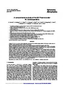
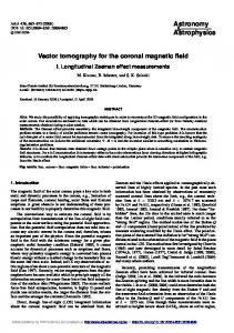
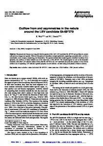
Fig. 1. Temporal evolution of the temperature and hydrogen density at the top of the loop for the two models.
3. Numerical results The hydrodynamics of the coronal plasma subject to a strong flaring heating has already been described extensively in previous papers in the literature. Here we dwell on the most important details. The evolution of the temperature and the density at the top of the loop are shown in Fig. 1. In the first minute of evolution, the coronal temperature increases from roughly 3 to 21 MK, for the model in which the energy is applied at the loop top (simulation A), and to around 15 MK for the model in which the energy is applied at the base of the TR (simulation B). During the early flare we find the largest differences between the two models. In both simulations A and B, the coronal density increases while the impulsive heating is on. After 200 s of the simulations, the hydrogen density at the top of the loop is of the order of 1017 m−3 . In the pre-flare conditions the plasma hydrogen density at the top of the loop was instead ∼7 × 10¹⁵ m−3 . As the coronal temperature increases, the conductive front propagates through the TR (the latter at the same time becomes steeper and steeper), and the chromospheric plasma warms up and, after ∼15 s, expands rapidly toward the corona (“chromospheric evaporation”).
In simulation A, velocities at temperatures above 106 K are always toward the loop top after the first 24 s and until the impulsive heating is active, i.e. until 360 s. In ∼30 s since the beginning of this simulation, the plasma velocity is ∼300 km s−1 in the corona. On the other hand, when the heating is applied at the base of the loop (simulation B), the plasma is pushed up since the very beginning and reaches velocities ∼400 km s−1 after 20 s. In both simulations a descendant flow of material occurs in the chromosphere, below the region being ablated and evaporated; there the plasma pressure is much lower than the pressure of the plasma evaporated in the corona and the material is shocked and compressed toward the bottom; velocities have much lower values than coronal ones. This process is generally called “chromospheric condensation” (Fisher 1987). As the plasma starts to evaporate, in both simulations the plasma temperature progressively increases along the whole loop; the emission measure at any temperature increases (as well as the EUV flux). The TR moves along the loop toward the foot-points during the whole heating phase. After 240 s, when the impulsive heating has decreased to around 1/3 of its maximum value, the corona
R. M. Betta et al.: Coronal loop hydrodynamics
starts to cool and the TR moves gradually back to its initial position. The simulations have been run to describe the plasma evolution for many minutes after the end of the heating. The loop cools and the coronal density decreases until a thermal instability (Field 1965) occurs: then the whole loop cools very rapidly and reaches typical chromospheric values (∼104 K). As a uniform and constant heating term (Hs ) is present in the equations, the whole loop returns approximately to its stationary pre-flare equilibrium after ∼3000 s. The entire cycle – until the whole coronal atmosphere returns exactly to the hydrostatic preflare conditions and the velocities decrease to negligible values – takes a few hours.
4. Light curves This flare has been described by MacNeice et al. (1985) and Cheng & Pallavicini (1988) (CP88, thereafter). We now summarize the most important features for a better comprehension of what is discussed in the following. It started at 17:00 UT and lasted less than 20 min. Four of the five instruments on board SMM registered the event: the Hard X-ray Burst Spectrometer (HXRBS), the Hard X-ray Imaging Spectrometer (HXIS), the X-ray Polychromator (XRP) and the Ultra-Violet Spectrometer and Polarimeter (UVSP). We concentrate on the observations made with the XRP (Acton et al. 1980) and with the UVSP (Woodgate et al. 1980). In Peres et al. (1987) the light curves from the whole raster in the X-ray lines observed with the XRP were compared with the results of the previous version of the PH code. An extensive analysis and interpretation of the hot component of this flare as well as of the spatial heating distribution and evolution was also included in that paper. During this flare the FCS instrument of the XRP registered spectroheliograms in six different resonance lines of some H-like ions or He-like: O viii 18.97 ˚ A (T ∼ 3 × 10⁶ K); Ne ix 13.45 ˚ A 6 (T ∼ 4 × 10 K); Mg xi 9.17 ˚ A (T ∼ 6.5 × 10⁶ K); Si xiii 6.65 ˚ A (T ∼ 107 K); S xv 5.04 ˚ A (T ∼ 1.55×10⁷ K); 7 Fe xxv 1.85 ˚ A (T ∼ 7 × 10 K). These lines covered most of the coronal temperature range. There are no qualitative differences between the light curves synthesized with the new and the previous version of the PH code, except the disappearance of the numerical noise which affected the results at the lowest coronal temperatures. Therefore we confirm that the previous simulations carried out by Peres et al. (1987) are adequate to model the X-ray line light curves. Here we focus most of our attention on the UVSP data. This spectrometer had good spectral resolution in the spectral band 1150–3600 ˚ A and spatial resolution better than 2 arcsec. The raster range was 256 × 256 arcsec2 . The UVSP collected images of this event with a field of view of 120 × 120 arcsec2 and pixels of 10 × 10 arcsec2 (i.e. ∼7250 × 7250 km2 on the Sun). Observations continued until the emitted flux increased considerably; since that moment (∼17:00:06 UT), rasters (a complete raster lasted
343
∼15 s) were alternated to spectral scans in two different lines, which lasted 30 s, with spectral resolution 0.3 ˚ A. These two lines, simultaneously recorded in two separate detectors, are ˚ line, formed at typical flaring plasma – Fe xxi 1354.1 A temperatures (T ∼ 107 K); – O v 1371.3 ˚ A line, formed at TR temperatures (T ∼ 2.2 × 10⁵ K). Both lines are partially blended with nearby lines (Feldman et al. 1977). The Fe xxi 1354.1 ˚ A line partially blends with the chromospheric C i 1355.844 ˚ A line; this C i line is very narrow (∼0.12 ˚ A), and, moreover, Cheng et al. (1979) showed that, during the flare maximum and decay phase, the intensity of the C i 1355.844 ˚ A line was ∼20% of the Fe xxi 1354.1 ˚ A line. The O v 1371.3 ˚ A line instead appeared blended with a very narrow line at 1371.37 ˚ A (not yet identified) during many flares observed by Skylab, which was not present in the quiescent phase (Feldman et al. 1977). The UVSP observed the rising phase in both lines. The flux in the O v 1371.3 ˚ A line, already high in the pre-flare phase, peaked at 17:02, i.e. at the same time as the peak observed in the hard X-rays. Then the emission in this line gradually decreased while the emission in the Fe xxi 1354.1 ˚ A line was still increasing (CP88). The light curve in the O v 1371.3 ˚ A line was different from the other ones observed simultaneously, because it peaked twice in the pre-flare phase (at 16:58 UT and at 16:59 UT) and, moreover, the flux was higher where a filament was observed in the Hα images. MacNeice et al. (1985) wrote that material expulsions appeared in this filament, at the velocity of 60 km s−1 before the rising phase of the flare. This filament disappeared after a short time and its disruption might be correlated to the increased emission in the O v 1371.3 ˚ A line. The light curves in the EUV lines recorded during this flare have been published in CP88. Cheng and Pallavicini distinguished three different zones in the flaring region, named as kernels F1, F2 and L1. The two kernels F1 and F2 covered the two foot-points of the loop while kernel L1 corresponded to the region between them, covering the top of the loop. The light curves in both lines were analyzed separately for each kernel as well as for the whole raster containing the entire flaring region, and are shown in Figs. 2–5. From the model results we calculate the flux in a particular line at a distance R from the Sun as Z s2 2A F = nne G(T )ds, (1) 4πR2 s1 where R is set equal to 1 AU in our calculations, A is the loop cross-section (assumed constant), G(T ) is the emission function tabulated by several authors for most observed lines, n is the hydrogen number density, ne the electron number density and s1 and s2 are the extreme loop points considered in the spatial integration; we multiply the flux by 2 because the loop is supposed to be
344
R. M. Betta et al.: Coronal loop hydrodynamics 10-3
Top heated loop Base heated loop
10-4
Flux [erg cm-2 s-1]
Flux [erg cm-2 s-1]
10-3
10-5
10-6 0
200
400 Time [s]
600
800
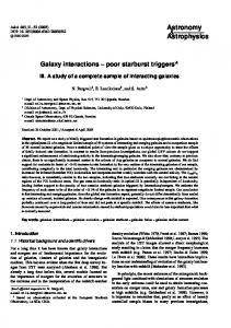
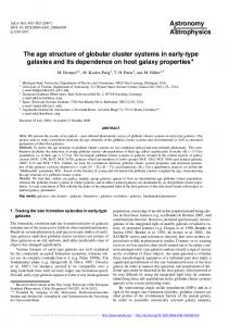
Fig. 2. Light curve observed in the Fe xxi 1354.1 ˚ A line by the UVSP/SMM in kernel L1 (solid line) from CP88. Also plotted are the light curves synthesized from hydrodynamic models with the emissivity tables computed by Monsignori Fossi (1994, private communication). In order to allow a proper comparison, the emission is integrated around the top of the loop.
symmetric and therefore the integral is evaluated on half a loop length. As a first step the integral [1] is calculated only in the loop volume corresponding to region L1 (two pixels). From Fig. 10 in CP88 we can guess that the loop was along the diagonal of kernel L1; assuming a semicircular geometry for the flaring coronal loop, and considering projection effects, the flux [1] is evaluated from s1 = 11 Mm to s2 = 20 Mm along half a loop, i.e. over a distance 9 Mm from the loop top. Results for He Fe xxi 1354.1 ˚ A are shown in Figs. 2 and 3 and are obtained using the tables for the emission function G(T ) calculated by Monsignori Fossi (1994, private communication). The observed light curve appears similar to those obtained for the X-ray lines with the FCS. This fact is not surprising as the FCS lines and the Fe xxi 1354.1 ˚ A line originate in the same part of the atmosphere. The curve computed with simulation B (base heating) is closer to the one observed during the flare onset, and the shape of the light curve is well simulated for the first 400 s. However the flux decreases too rapidly during the flare decay. On the other hand, with the heating at the top (simulation A), the curve is too low during the early phase, but it is high even well after the heating is switched off. The modeled light curve peaks later than the observed one, but follows the flare decay emission better, even though also model A predicts a more rapid decrease of the intensity than observed, implying that further heating might be released during the flare decay in the EUV emitting plasma. In Fig. 3 the emission integrated over the whole loop is compared with the flux in the Fe xxi 1354.1 ˚ A line coming from the whole raster for both the simulations. The modeled curves are now very different from the observed
Top heated loop Base heated loop
10-4
10-5
10-6 0
200
400 Time [s]
600
800
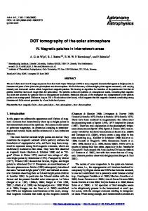
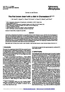
˚ line observed by Fig. 3. Light curve in the Fe xxi 1354.1 A the UVSP/SMM in the whole raster (solid line) from CP88. Also plotted are the light curves synthesized with our code and with the emissivity tables computed by Monsignori Fossi (1994, private communication) for both models. The line emission is integrated along the whole loop.
one, as the total measured intensity is much higher than the calculated one in both cases. The observed emission in the O v 1371.3 ˚ A line was brighter in both kernels F1 and F2, corresponding to the two foot-points of the loop, than elsewhere in the raster region. A chromospheric filament was probably responsible for the initially increased emission in kernel F2 during the pre-flare phase (see above). The observed flux in region F2 is higher than in F1 and the two light curves are different (see CP88, Fig. 10), suggesting the presence of other emitting chromospheric structures in region F2. For this reason we have compared our calculations only with the data of kernel F1 and not with those of F2. In kernel F1 there is high pre-flare emission, which could be related to the presence of other closed structures emitting in the O v 1371.3 ˚ A line or in the blended unidentified line mentioned above. From our hydrodynamic calculations we simulate the light curve in this line using two different formulations for the emissivity G(T ): 1. the spectral emission function tabulated by Landini & Monsignori Fossi (1990) and following upgrades (thereafter LMF); 2. the emissivity computed with Raymond’s spectral code (Raymond & Smith 1977, and following upgrades, henceforth RS). The two modeled light curves have the same profile but they differ by almost one order of magnitude. Discrepancies in the results obtained with different spectral models have already been pointed out by Pallavicini (1994) and constitute an important difficulty in comparing real data with the hydrodynamic calculations or any other modeling results. Anyway, the discrepancy among spectral models does not significantly alter the shape of the light curve, but mostly the intensity.
R. M. Betta et al.: Coronal loop hydrodynamics 10-3 Top heated loop
Top heated loop
Base heated loop
Base heated loop Flux [erg cm-2 s-1]
Flux [erg cm-2 s-1]
10-3
10-4
10-5 0
200
400 Time [s]
600
800
200
400 Time [s]
600
800
10-3 Top heated loop
Top heated loop
Base heated loop
Base heated loop Flux [erg cm-2 s-1]
Flux [erg cm-2 s-1]
10-4
10-5 0
10-3
10-4
10-5 0
345
200
400 Time [s]
600
800
10-4
10-5 0
200
400 Time [s]
600
800
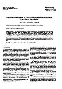
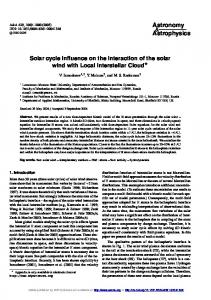
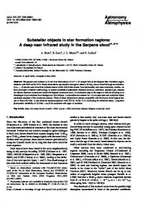
˚ line of kernel F1 Fig. 4. The emission in the O v 1371.3 A (covering one foot of the loop) is compared with the results of our two numerical calculations and the LMF spectral synthesis model (top). In the plot at the bottom the same results are shown together with the flux emitted from the whole raster (CP88).
Fig. 5. The emission of kernel F1 (covering one foot of the loop) is compared with the results of our two numerical calculations and the spectral synthesis model RS (top). In the plot at the bottom the flux emitted from the whole raster (CP88) is compared with the same modeled curves.
We have first compared the flux integrated over half a loop with the emission from kernel F1; as a matter of fact, according to our model, only the TR contributes to the emission in the O v 1371.3 ˚ A line, and therefore, only the foot-points of the loop are bright in this wavelength. In Fig. 4 and in Fig. 5 we compare our numerical results (both simulations A and B) with the observed flux in kernel F1 (top panel). We also plot the light curves predicted by our hydrodynamic calculations and the measured flux coming from the whole raster (bottom panel). The raster flux is larger than that predicted with a single loop model, either if we assume the LMF spectral model or the RS model. This fact is not surprising because many other structures present in the raster might contribute to the emission, as for the Fe xxi 1354.1 ˚ A line. Results obtained with the RS spectral model are in better agreement with the observations in kernel F1. The O v 1371.3 ˚ A line peaks earlier than the Fe xxi 1354.1 ˚ A line in our simulations as well as in the
real observation but the O v 1371.3 ˚ A light curves of our models are qualitatively different from the data plotted in CP88, at least for the first 5 min. The model with the heating at the loop top and the RS spectral model approximate the decay light curve quite well. This could be said also for the bottom heated model for t < 700 s. Then a thermal instability occurs (see long-dashed lines in Fig. 4 and in Fig. 5). The rapid cooling of the atmosphere, mostly due to the increase of radiative losses as the temperature decreases below 106 K, determines a significant peak of the emission which makes model B unlikely to describe this flare.
5. Discussion and conclusions The X-ray emission of this flaring loop has been accurately modeled by Peres et al. (1987) using the hydrodynamic results of the PH code: in that work they obtained theoretical light curves very close to the observed ones.
346
R. M. Betta et al.: Coronal loop hydrodynamics
In this paper we compare the results of our numerical calculations with both typical TR emission and coronal ones, simultaneously. From the analysis of all the modeled light curves in both the X-rays and EUV bands and the data registered during the event, we note that the top heated loop model gives results in better agreement with the coronal emission than the bottom heated loop model, during the entire flare evolution, in agreement with Peres et al. (1987). On the basis of our new calculations we can add that this model also accounts for the observed Fe xxi 1354.1 ˚ A line during a large fraction of the November 12, 1980 flare. We note that the computed light curves in the Fe xxi 1354.1 ˚ A line have a shape similar to those of the X-ray lines formed in the same temperature range, and therefore originating from the same part of the atmosphere. Both our models predict Fe xxi line flux close to the observed one at the time of the flare X-ray line peak, which occurred during the decay of the flare light curve in the observed O v 1371.3 ˚ A line. Also the top-heated model yields an already decaying OV light curve at the time of coronal lines flare maximum. However during the early flare the lower TR emission cannot be fitted with the same model which consistently yields lower emission than observed. This suggests that more plasma than modeled might have contributed to the O v 1371.3 ˚ A line emission. In summary, the analysis of the hot coronal EUV emission (Fe xxi 1354.1 ˚ A line) confirms the scenario derived with the previous study (Peres et al. 1987) based on X-ray lines. The study of the O v 1371.3 ˚ A line, instead, shows a rather different evolution and the relevant light curve is poorly fitted by the hydrodynamic loop model which instead works well for the hot coronal emission. We therefore confirm that the single loop model (albeit a schematic approximation of reality) works well for the corona of this flare, and therefore that a single loop – or a bundle of loops evolving coherently – dominated the coronal emission, as MacNeice et al. (1985) and Peres et al. (1987) suggested. The colder plasma emission, instead, appears dominated by other structures, probably some already present at an earlier phase, others evolving and reaching their maximum emission before the Fe xxi 1354.1 ˚ A line peak. Also Feldman (1983), Widing & Cook (1987), Doschek (1997), Mason (1998) observed that there is a mismatch between TR and coronal flare emission.
It appears that a single loop model is not adequate to fit the lower TR lines simultaneously to the coronal lines (which are well fitted), at least for this flare. To this end more complex models may be required, such as multistructure models. Acknowledgements. This work has been done with partial support of the Italian Ministero dell’Universit` a e della ricerca Scientifica e Tecnologica and of the Agenzia Spaziale Italiana.
References Acton, L. W., Culhane, J. L., Gabriel, A. H., et al. 1980, Solar Phys., 65, 53 Betta, R., Peres, G., Reale, F., & Serio, S. 1997, A&AS, 122, 585 Cheng, C. C., Feldman, U., & Doscheck, G. A. 1979, ApJ, 233, 736 Cheng, C. C., & Pallavicini, R. 1988, ApJ, 324, 113 Doschek, G. A. 1997, ApJ, 476, 903 Feldman, U. 1983, ApJ, 275, 367 Feldman, U., Doscheck, G. A., & Rosenberg, F. D. 1977, ApJ, 215, 652 Field, G. B., ApJ, 142, 531 Fisher, G. H. 1987, ApJ, 317, 502 Landini, M., & Monsignori Fossi, B. C. 1990, A&AS, 82, 229 MacNeice, P., Pallavicini, R., Mason, H. E., et al. 1985, Solar Phys., 99, 167 Maggio, A., Reale, F., Peres, G., & Ciaravella, A. 1994, Comp. Phys. Comm., 81, 105 Mason, H. E. 1998, J. Phys. Colloq. France, 49, C1–13 Pallavicini, R. 1994, Spectroscopic Diagnostics of Astrophysical Plasmas, in Plasma Astrophysics, Lectures held at the Astrophysics School VII Organized by the European Astrophysics Doctoral Network (EADN), San Miniato, 4–14 October 1994, ed. by C. Chiuderi, & G. Einaudi Peres, G. 2000, Solar Phys., 193, 33 Peres, G., Reale, F., Serio, S., & Pallavicini, R. 1987, ApJ, 312 895 Peres, G., Rosner, R., Serio, S., & Vaiana, G. S. 1982, ApJ, 252 791 Reale, F., Peres, G., Serio, S., Betta, R., DeLuca, E. E., & Goulb, L. 2000, ApJ, 535 423 Raymond, J. C., & Smith, B. W. 1977, ApJS, 35 419 Widing, K. G., & Cook, J. W. 1987, ApJ, 320 913 Woodgate, B. E., Tandberg-Hanssen, E. A., et al. 1980, Solar Phys., 65 73