KEY WORDS: Computer experiment; Design of experiments; Asymmetric ... We propose an approach for constructing asymmetric nested lattice samples by .... d matrix, where the first d1 columns take values from a set of s1 levels, the next d2.
Asymmetric Nested Lattice Samples Peter Z. G. Qian1 and Mingyao Ai2,3 1
Department of Statistics
University of Wisconsin-Madison, Madison, WI 53706 2
LMAM, School of Mathematical Sciences Peking University, Beijing 100871, China 3
Corresponding author
KEY WORDS: Computer experiment; Design of experiments; Asymmetric orthogonal array; Orthogonal array based Latin hypercube; Sequential design; Space-filling design; Randomized orthogonal array. Abstract We propose an approach for constructing asymmetric nested lattice samples by randomizing asymmetric nested orthogonal arrays. Such designs possess a desirable nested structure and have attractive space-filling properties. Unlike recently developed symmetric nested lattice samples, different axes of asymmetric nested lattice samples can be divided at different scales of fineness. The proposed designs are motivated by the problem of running multi-fidelity computer experiments and also are useful for sequential evaluation of complex computer codes, and calibration and validation of computer models.
1
INTRODUCTION
Multi-fidelity computer modeling is a vital tool for studying complex systems in sciences and engineering. Typically this strategy first conducts a low-accuracy computer experiment with a large number of runs and a high-accuracy computer experiment with a smaller number of runs, and then combines the two sets of results together for metamodeling, optimization and other purposes. Following Qian and Wu (2008), the two experiments are denoted by LE and HE, where HE is more accurate than LE but also more expensive to run. The pair can be a 1
finite element analysis model vs. a finite difference model, or a computational fluid dynamics (CFD) model with high resolution vs. a CFD model with low resolution. Such experiments have recently become prevalent in a wide array of fields, such as conceptual design, electronic cooling, food engineering (Dewettinck et al. 1999), hydrology, nanotechnology oil reserve management, fuel cells manufacturing (Wang and Wang 2006). For illustration, two examples from engineering are described below.
(a)
(b)
Figure 1: (a) A Heat Transfer Device for an Electronic Cooling Application (Qian et al. 2006) and (b) a Mining Crawler (Negrut, Qian, and Khude 2007).
Example 1. Qian et al. (2006) used multi-fidelity computer experiments to study the thermal dynamics in a heat exchanger for a representative electronic cooling application. The mechanism for heat dissipation is forced convection with air as the working fluid. Figure 1(a) shows a heat exchanger, which is a linear cellular alloy with ordered, extended prismatic channels. The response of interest is the heat transfer rate in the heat exchanger. Five design factors can potentially affect the thermal process. Two types of computer experiments — an HE based on computationally expensive finite element simulations and an LE based on relatively fast but more approximate finite difference simulations — are used to analyze the impact of these factors on the heat transfer rate. The HE and LE have different levels of accuracy and computational times: each HE run requires two orders of magnitude more computing time than the corresponding LE run; and the HE runs are more accurate than the LE runs by 2
10%. Example 2. Figure 1(b) shows a mining crawler, a subcomponent of a low-mobility hydraulic mining excavator, taken from Negrut, Qian and Khude (2007). Two types of Index 3 Differential Algebraic Equations computer experiments are used to model the multibody dynamics of this crawler. An HE is based on an ODE type MATLAB program using a fourth order Runge-Kutta method that can precisely compute the time evolution of the slider-crank. An LE is based on an MSC.ADAMS program (MSCsoftware, 2005) that uses implicit integration formulas to approximate the time evolution of the multibody system. The issue of modeling data from a pair of HE and LE has attracted a recent surge of interests in statistics. Related work includes Kennedy and O’Hagan (2000, 2001), Reese et al. (2004), Qian et al. (2006), Higdon et al. (2008), and Qian and Wu (2008), among others. Most of these methods are based on Gaussian process models (Sacks et al. 1989; Santner, Williams, and Notz 2003; Fang, Li, and Sudjianto 2005). Because the HE is more accurate than the LE, the objective is to obtain a prediction model that can produce results close to the HE. This is achieved by first fitting a statistical model to the LE data and then refining it using the HE data to better predict the HE. It is intuitively appealing to use nested space-filling designs (NSFD’s) to collect data from a pair of HE and LE for the purpose of building an accurate prediction model for the HE. A pair of NSFD’s are two space-filling designs in which the smaller design is nested within the large design. Existing classes of NSFD’s include nested Latin hypercube designs (Qian 2009) and those based on level-projection nested orthogonal arrays (Qian, Tang, and Wu 2009; Qian, Ai, and Wu 2009). A level-projection nested orthogonal array is an orthogonal array that contains a subarray that itself becomes an orthogonal array after the levels are collapsed according to a projection from a large Galois field to a small Galois field. The subarray is not necessarily an orthogonal array before the level projection. NSFD’s can also be obtained from nets (Niederreiter 1992; Owen 1995) and orthogonal Latin hypercube designs (Ye 1998; Steinberg and Lin 2006; Bingham, Sitter, and Tang 2009; Lin, Mukerjee, and Tang 2009) . By randomizing nested orthogonal arrays, Qian and Ai (2010) introduced 3
a new type of NSFD, called nested lattice samples (NLS’s). NLS’s extend earlier work on orthogonal array based sampling designs (Patterson 1954; Owen 1992; Tang 1993). A pair of NLS’s associated with a nested orthogonal array with strength t has a desirable nested structure and possesses attractive space-filling properties in that the points in both designs achieve uniformity in both t or lower dimensions. NLS’s constructed in Qian and Ai (2010) are based on symmetric nested orthogonal arrays and hence are symmetric in the sense all axes of such designs are divided at the same scale of fineness. In this article, we construct asymmetric NLS’s in which different axes can be divided at different scales of fineness. Unlike Qian and Ai (2010), our construction here is based on asymmetric nested orthogonal arrays. The remainder of the article will unfold as follows. A formal definition of asymmetric nested orthogonal array is presented in Section 2. Two approaches for constructing asymmetric NOA’s are given in Sections 3. A procedure for generating asymmetric NLS’s by randomizing asymmetric NOA’s with nested permutations is presented in Section 4. A short summary and discussions is provided in Section 5.
2
DEFINITIONS AND NOTATION
This section gives some useful definitions and notation. A symmetric orthogonal array (OA) of size n, m constraints, s levels, and strength two, denoted by OA(n, sm , 2), is an n × m matrix with entries from a set of s levels, such that, for every n × 2 submatrix, each of the s2 level combinations occurs equally often (Hedayat, Sloane, and Stufken 1999, HSS hereinafter). Throughout, we consider only OA’s of strength two and drop the third parameter in OA(n, sm , 2). Mukerjee, Qian, and Wu (2008) introduced the concept of nested orthogonal arrays (NOA’s), which is related to that of incomplete orthogonal arrays (Hedayat and Stufken 1992). An NOA OA((n1 , n2 ), (sd1 , sd2 )) is an OA(n1 , sd1 ) containing an OA(n2 , sd2 ) as a subarray, where n1 > n2 and s1 > s2 . Several construction methods for symmetric NOA’s were developed in Qian and Ai (2010). It is also possible to generate such arrays from ordered orthogonal arrays (Sch¨ urer and Schmid 2010). For illustration, Table 1 presents an OA((16, 4), (43 , 23 )). 4
0101 001122223333
0011 232301230123 0110 233223013210
Table 1: An OA((16, 4), (43 , 23 )) (in transpose), where the first four rows form an OA(4, 23 ) We now give a formal definition of asymmetric NOA’s. Recall that an asymmetric Pv orthogonal array OA(n, sd11 · · · sdvv ) of size n and strength two, d = i=1 di , is an n × d matrix, where the first d1 columns take values from a set of s1 levels, the next d2 columns take values from a set of s2 levels and so on, such that, for every n × 2 submatrix, all possible level combinations occur equally often. For n2 < n1 and si2 ≤ si1 , i = 1, . . . , v, suppose that A is an OA(n1 , sd111 · · · sdv1v ) containing a submatrix, B, that forms an OA(n2 , sd121 · · · sdv2v ). Then A, or more precisely B ⊂ A, is called an asymmetric NOA, denoted by OA((n1 , n2 ), (sd111 · · · sdv1v , sd121 · · · sdv2v )), where s11 , . . . , sv1 are all distinct but some of the parameters s12 , . . . , sv2 could be identical. For v = 1, an OA((n1 , n2 ), (sd111 · · · sdv1v , sd121 · · · sdv2v )) reduces to an OA((n1 , n2 ), (sd11 , sd12 )).
3
CONSTRUCTION OF ASYMMETRIC NOA’S
3.1
A Level-collapsing Approach
The idea of level collapsing has been used for constructing asymmetric OA’s (HSS). By extending this idea, we propose an approach for constructing asymmetric NOA’s that collapses the levels of a symmetrical NOA in an elaborate manner to form an asymmetric NOA. Let B ⊂ A be an OA((n1 , n2 ), (sd1 , sd2 )). Suppose that r1 and r2 are integers with s1 > r1 > s2 ≥ r2 , r1 |s1 and r2 |s2 . We now present a scheme to collapse the levels of any factor in B ⊂ A to r1 and r2 levels for A and B, respectively. This scheme has two steps. Grouping: Partition the s1 levels of a factor in A into r1 groups of size s1 /r1 , such that the s2 levels of the factor in B are partitioned into r2 groups of size s2 /r2 .
5
Collapsing: Replace all symbols in each of the r1 groups associated with the factor in A by a new common symbol. For i = 1, . . . , d, let B∗ ⊂ A∗ denote the resulting pair of arrays after the foregoing scheme is successively applied to i factors of B ⊂ A. Proposition 1. Consider the pair of arrays A∗ and B∗ constructed above. Then we have that i a. the matrix A∗ is an OA(n1 , sd−i 1 r1 );
b. the matrix B∗ is a submatrix of A∗ , and B∗ is an OA(n2 , s2d−i r2i ). This proposition follows by noting that the forgoing scheme does not affect the orthogonality and nesting of B ⊂ A. Example 3. For s1 = 16 and s2 = 4, let B ⊂ A be an OA((256, 16), (165 , 45 )) constructed in Qian and Ai (2010) by using the Rao-Hamming method (HSS) under a subfield condition. Table 2 presents the array B, which is an OA(16, 45 ). Here, the four levels of B are 0, 1, 2, 3, and the 16 levels of A are 0, 1, . . . , 15.
0101001122223333
0011232301230123 0110233223013210 0123312020133102 0132120321303021
Table 2: The array B (in transpose ) in Example 3, which is an OA(16, 45 ) Let r1 = 8 and r2 = 2. The first step of the forgoing scheme partitions the 16 levels of any factor in A into 8 groups of size 2, given as {2j − 2, 2j − 1}, j = 1, . . . , 8, where the four levels, 0, 1, 2, 3, of the corresponding factor in B are located in the first two groups, {0, 1} and {2, 3}, each of size two. For j = 1, . . . , 8, the second step of the forgoing scheme collapses the two levels 2j − 2 and 2j − 1 of group j into j − 1. Applying this scheme to factor 6
1 of B ⊂ A gives an OA((256, 16), (81 164 , , 21 44 ), denoted by B∗ ⊂ A∗ . Table 3 presents the array B∗ , which is an OA(16, 21 44 ).
0000000011111111
0011232301230123 0110233223013210 0123312020133102 0132120321303021
Table 3: The array B∗ (in transpose) in Example 3, which is an OA(16, 21 44 ) For i = 1, . . . , 5, successively apply this scheme to i factors in B ⊂ A gives an OA((256, 16), (8i 165−i , 2i 45−i )). Example 4. For s1 = 8 and s2 = 2, let B ⊂ A be an OA((64, 4), (83 , 23 )) from Table 4. Let r1 = 4 and r2 = 2. The first step of the forgoing scheme partitions the eight levels of A into four groups, {0, 4}, {1, 5}, {2, 6}, {3, 7}, and the second step of the scheme collapses the two levels of the four groups into 0, 1, 2, 3, respectively. Applying this scheme to factor 3 of A gives an OA((64, 4), (82 41 , 23 ), denoted by B∗ ⊂ A∗ . Table 5 presents the pair of arrays B∗ ⊂ A∗ .
0011 000000111111222222223333333344444444555555556666666677777777
0101 234567234567012345670123456701234567012345670123456701234567 0110 234567325476230167453210765445670123547610326745230176543210
Table 4: An OA((64, 4), (83 , 23 )) (in transpose) in Example 4, where the first four rows form an OA(4, 23 ) Now, for any integers m2 > m1 ≥ 2, let B ⊂ A be an OA(((m1 m2 )2 , m21 ), ((m1 m2 )3 , m31 )) from Example 4 of Qian and Ai (2010). For i = 1, 2, 3, by collapsing the m1 m2 levels of i factors in A into m2 levels as done above, an OA(((m1 m2 )2 , m21 ), ((m1 m2 )3−i mi2 , m31 )) is constructed.
7
0011 000000111111222222223333333344444444555555556666666677777777
0101 234567234567012345670123456701234567012345670123456701234567 0110 230123321032230123013210321001230123103210322301230132103210
Table 5: An OA((64, 4), (82 41 , 23 )) (in transpose) in Example 4, where the first four rows form an OA(4, 23 )
3.2
A Replacement Approach
Here we propose another approach for constructing asymmetric NOA’s that employs the method of replacement (HSS). Let B ⊂ A be an OA((n1 , n2 ), (sd1 , sd2 )) and let V ⊂ W be an OA((s1 , s2 ), (r1m , r2m )). We now present a scheme to replace any factor at s1 and s2 levels for A and B with m new factors at r1 and r2 levels for A and B, respectively. This scheme has two steps. Labeling: Label the s1 rows of W by the s1 symbols of a factor for A, such that the s2 rows of V are labeled by the s2 symbols of the factor for B. Replacing: Replace each symbol of the factor for A with the row of W labeled by the symbol. For i = 1, . . . , d, let B∗ ⊂ A∗ denote the resulting pair of arrays after the foregoing scheme is successively applied to i factors of B ⊂ A. Proposition 2. Consider the pair of arrays A∗ and B∗ constructed above. Then we have that im a. the matrix A∗ is an OA(n1 , sd−i 1 r1 );
b. the matrix B∗ is a submatrix of A∗ , and B∗ is an OA(n2 , s2d−i r2im ). This proposition follows by noting that the forgoing scheme does not affect the orthogonality and nesting of B ⊂ A.
8
Example 5. Let B ⊂ A be an OA((256, 16), (165 , 45 )) from Example 3, and let V ⊂ W be an OA((16, 4), (43 , 23 )) from Table 1. Here, the four levels of B are 0, 1, 2, 3, and the 16 levels of A are 0, 1, . . . , 15. The first step of the forgoing scheme labels the 16 rows of W, given in Table 1, by the symbols 0, 1, . . . , 15 of A, such that the four rows of V correspond to the symbols 0, 1, 2, 3 of B. For j = 0, 1, . . . , 15, the second step of the forgoing scheme replaces each symbol j of any column in B ⊂ A with the row of W labeled by j. Then the factor of B ⊂ A is replaced with three new factors with 4 and 2 levels for A and B, respectively, resulting in an OA((256, 16), (43 164 , 23 44 )). Applying this scheme to factor 1 of B ⊂ A gives an OA((256, 16), (43 164 , 23 44 )), denoted by B∗ ⊂ A∗ . Table 6 presents the array B∗ , which is an OA(16, 23 44 ). 0101001100001111
0000000011111111 0101001111110000 0011232301230123 0110233223013210 0123312020133102 0132120321303021
Table 6: The array B∗ (in transpose) in Example 5, which is an OA(16, 23 44 ) Similarly, for i = 2, . . . , 5, using such replacement for i factors of A gives an OA((256, 16), (43i 165−i , 23i 45−i )). Example 6. Let B ⊂ A be an OA((6561, 81), (8110 , 910 )) and V ⊂ W be an OA((81, 9), (94 , 34 )) from Proposition 1 of Qian and Ai (2010) constructed by using the Rao-Hamming method under a subfield condition. Table 7 presents the pair of arrays V ⊂ W. Here, the eight levels in B are 0, 1, . . . , 8 and the 81 levels in A are denoted by 0, 1, . . . , 80. Label the 81 rows of W by the symbols 0, 1, . . . , 80 of A, such that the nine rows of V correspond to the symbols 0, 1, . . . , 8 of B. For i = 1, . . . , 10, by replacing each symbol j of i factors in A with the row of W labeled by j, an OA((6561, 81), (94i 8110−i , 34i 910−i )) is obtained. 9
000111222 345678345678345678012345678012345678012345678012345678012345678012345678
012012012 000000111111222222333333333444444444555555555666666666777777777888888888 012120201 345678453786534867345678012453786120534867201678012345786120453867201534 021102210 345678534867453786678012345867201534786120453345678012534867201453786120
Table 7: An OA((81, 9), (94 , 34 )) (in transpose) in Example 6, where the first nine rows form an OA(9, 34 )
4
GENERATION OF ASYMMETRIC NESTED LATTICE SAMPLES
In this section, we present a procedure for generating a pair of asymmetric NLS’s by randomizing an asymmetric NOA with nested permutations. This procedure extends the one used in Qian and Ai (2010) in order to cover asymmetric NOA’s. Here are some additional definitions and notation. A uniform permutation on a set of p integers is a permutation on the set, with all p! possible permutations being equally probable. For a ∈ R, dae denotes the smallest integer no less than a. For an integer m ≥ 1, Zm denotes the set {1, . . . , m}. Let a > b ≥ 1 be two integers with b|a and let c = a/b. Following Qian (2009), a nested permutation π a,b np = π np = (πnp (1), . . . , πnp (a)) is generated as follows. Step 1: Draw a uniform permutation λ = (λ(1), . . . , λ(b)) on Zb . Step 2: For i = 1, . . . , b, draw πnp (i) from Udis [(λ(i) − 1)c + 1, λ(i)c], which denotes the discrete uniform distribution with support {λ(i) − 1)c + 1, · · · , λ(i)c}. Step 3: Obtain (πnp (b + 1), . . . , πnp (a)) as a uniform permutation on the intersection of Za and the set theoretic complement of {πnp (1), . . . , πnp (b)}. The term “nested permutation” suggests that, concerning the first b elements of a π a,b np , (dπnp (1)/ce, . . . , dπnp (b)/ce) constitute a permutation on Zb . Such a permutation is essentially Owen’s randomization method for nets (Owen 1995). 10
Let V ⊂ W be an OA((n1 , n2 ), (sd111 · · · sdv1v , sd121 · · · sdv2v )) with d =
Pv
k=1
dv . Let ak denote
the number of levels of the kth column of W and bk denote the number of levels of the kth column of V. For k = 1, . . . , d, we first relabel the levels of the kth column of W in such a way that the s1 levels become 1, . . . , s1 , and the s2 levels of B become 1, . . . , s2 . Since V is a subset of W, this relabeling changes the levels of V as well. It needs to be stressed here that the pair of nested arrays V ⊂ W does not automatically generate a pair of nested samples with good space-filling properties if the s1 levels are randomized with uniform permutations on Zs1 . Though such level permutation will give a design that achieves uniformity in two dimensions, the subset of points of the design corresponding to V may not have good spacefilling properties. For k = 1, . . . , d, the key here is to use a nested permutation π anpk ,bk to permute the ak levels of the kth column of W, such that, after the randomization, one and only one of the bk levels of V falls within each of the bk blocks defined by 1, . . . , qk ; qk + 1, . . . , 2qk ; . . . ; (bk − 1)qk + 1, . . . , bk qk , where qk = ak /bk . Precisely, a pair of asymmetric nested lattice samples based on V ⊂ W is generated as follows. Obtain an n1 × d array D1 through xik = a−1 k [ηk (wik ) − uik ], i = 1, . . . , n1 , k = 1, . . . , d,
(1)
where wik is the (i, k)th entry of W, xik is the (i, k)th entry of D1 , η k is a nested permuak ,bk tation πnp , all the η k are obtained independently, the uik are independent U [0, 1] random
variables, and the η k and the uik are mutually independent. Let D2 be the subset of points in D1 corresponding to V. Then D2 ⊂ D1 provide a pair of asymmetric NLS’s with attractive stratification in which different axes can be divided at different levels of fineness. We make this precise in Proposition 3. Proposition 3. Consider D2 ⊂ D1 constructed above. Then we have that a. the array D1 achieves stratification on ak1 ×ak2 grids when projected onto factors k1 , k2 ; b. the array D2 achieves stratification on bk1 ×bk2 grids when projected onto factors k1 , k2 .
11
Example 7. Let V ⊂ W be the OA((64, 4), (82 41 , 23 )) from Table 5. Relabel the levels 0, 1, 2, . . . , 7 of W as 1, 2, 3, . . . , 8, respectively, where the levels of V become 1 and 2. A pair of asymmetric NLS’s, D2 ⊂ D1 , is generated by using two independent nested permutation 8,2 to randomize the levels of the first two columns of W and a nested permutation π 4,2 π np np to
randomize the levels of the third column of W. The bivariate projections of D1 are plotted in Figure 2, where the points are evenly distributed on 8 × 8 grids in the dimensions of factors 1 and 2, on 8 × 4 grids in those of factors 1 and 3, and on 8 × 4 grids in those of factors 2 and 3. Figure 3 depicts the bivariate projections of D2 , where the points are evenly scattered on 2 × 2 grids in any two dimensions.
0.2
0.4
0.6
0.8
1.0
0.6
0.8
1.0
0.0
0.6
0.8
1.0 0.0
0.2
0.4
x1
0.8 0.6
0.6
0.8
1.0
1.0 0.0
0.2
0.4
x2
0.4 0.2 0.0
0.0
0.2
0.4
x3
0.0
0.2
0.4
0.6
0.8
1.0 0.0
0.2
0.4
0.6
0.8
1.0 0.0
0.2
0.4
0.6
0.8
1.0
Figure 2: Bivariate projections of D1 associated with the asymmetric NOA in Table 5
12
0.2
0.4
0.6
0.8
1.0
0.6
0.8
1.0
0.0
0.6
0.8
1.0
0.0
0.2
0.4
x1
1.0 0.8 0.6
0.6
0.8
1.0
0.0
0.2
0.4
x2
0.4 0.2 0.0
0.0
0.2
0.4
x3
0.0
0.2
0.4
0.6
0.8
1.0
0.0
0.2
0.4
0.6
0.8
1.0
0.0
0.2
0.4
0.6
0.8
1.0
Figure 3: Bivariate projections of D2 associated with the asymmetric NOA in Table 5
13
5
SUMMARY AND DISCUSSION
We have proposed a method for randomizing asymmetric nested orthogonal arrays with nested permutations to generate asymmetric nested lattice samples. Two easy-to-implement approaches have been developed for constructing asymmetric nested orthogonal arrays. The constructed designs are also useful for estimating the mean of the outputs from a pair of HE and LE given a distribution of inputs (McKay, Conover, and Beckman 1979; Qian 2009). Other potential applications of asymmetric nested lattice samples include sequential evaluation of complex computer codes and calibration and validation of computer models (Kennedy and O’Hagan 2001; Loeppky, Bingham, and Welch 2010). Beyond computer experiments, such designs can be used for sequentially approximating multi-dimensional integrals for the Monte Carlo EM algorithm, stochastic programs and chance-constraint problems. By replacing random nested permutations in (1) with more sophisticated level permutation schemes, it is possible to generate optimal asymmetric nested lattice samples guided by either the minimax or maximin distance criterion (Tang 1994; Leary, Bhaskar, and Keane 2003). Because the constructed asymmetric NOA’s in Section 3 have strength two, their corresponding asymmetric nested lattice samples are guaranteed to achieve uniformity in two dimensions only. To generate asymmetric nested lattice samples with better space-filling properties, we plan to develop methods to construct asymmetric NOA’s with strength three or higher in the future. ACKNOWLEDGEMENTS Qian is supported by NSF Grants DMS-0705206 and CMMI-0969616, and a faculty award from IBM, and Ai is supported by NNSF of China Grant 10971004 and NBRP of China Grant 2007CB512605.
14
References Bingham, D., Sitter, R. R., and Tang, B. (2009), “Orthogonal and Nearly Orthogonal Designs for Computer Experiments,” Biometrika, 96, 51–65. Dewettinck, K., Visscherb, A. D., Derooa, L., and Huyghebaert, A. (1999). “Modeling the Steady-state Thermodynamic Operation Point of Top-spray Fluidized Bed Processing,” Journal of Food Engineering, 39, 131–143. Fang, K. T., Li, R. Z., and Sudjianto, A. (2005), Design and Modeling for Computer Experiments, New York: Chapman and Hall/CRC Press. Hedayat, A. S., Sloane, N. J. A., and Stufken, J. (1999), Orthogonal Arrays: Theory and Applications, New York: Springer. Hedayat, A. S., and Stufken, J. (1992), “Some Mathematical Results on Incomplete Orthogonal Arrays,” Sankhya, Ser A, 54, 197–202. Higdon, D., Gattiker, J., Williams, B., and Rightley, M. (2008), “Computer Model Calibration Using High-Dimensional Output,” Journal of the American Statistical Association, 103, 570–583. Kennedy, M. C., and O’Hagan, A. (2000), “Predicting the Output from a Complex Computer Code When Fast Approximations Are Available,” Biometrika, 87, 1–13. Kennedy, M. C., and O’Hagan, A. (2001), “Bayesian Calibration of Computer Models,” Journal of the Royal Statistical Society, Ser B, 63, 425–464. Leary, S., Bhaskar, A., and Keane, A. (2003), “Optimal orthogonal-array-based Latin hypercubes,” Journal of Applied Statistics, 30, 585598. Lin, C. D., Mukerjee, R., and Tang, B. (2009), “Construction of Orthogonal and Nearly Orthogonal Latin Hypercubes,” Biometrika, 96, 243–247.
15
Loeppky, J. L., Bingham, D., and Welch, W. J. (2010), Computer Model Calibration or Tuning in Practice, Technical Report. McKay, M. D., Conover, W. J., and Beckman, R. J. (1979), “A Comparison of Three Methods for Selecting Values of Input Variables in the Analysis of Output from a Computer Code,” Technometrics, 21, 239–245. MSCsoftware (2005), ADAMS User Manual, Available at http://www.mscsoftware.com. Mukerjee, R., Qian, P. Z. G., and Wu, C. F. J. (2008), “On the Existence of Nested Orthogonal Arrays,” Discrete Mathematics, 308, 4635–4642. Negrut, D., Qian, P. Z. G., and Khude, N. (2007),“Building Gaussian Process Based Metamodels Using Variable-fidelity Experiments for Dynamic Analysis of Mechanical Systems,” Proceedings of the 2007 ASME International Mechanical Engineering Congress and Exposition, Seattle, WA. Niederreiter, H. (1992), Random Number Generation and Quasi-Monte Carlo Methods, Philadelphia: Society for Industrial Mathematics. Owen, A. B. (1992), “Orthogonal Arrays for Computer Experiments, Integration and Visualization,” Statistica Sinica, 2, 439–452. Owen, A. B. (1995), “Randomly Permuted (t, m, s)-nets and (t, s)-sequences,” in Monte Carlo and Quasi-Monte Carlo Methods in Scientific Computing, Lecture Notes in Statistics, 106, 299–317, New York: Springer. Patterson, H. D. (1954), “The Errors of Lattice Sampling,” Journal of the Royal Statistical Society, Ser B, 16, 140–149. Qian, P. Z. G. (2009), “Nested Latin Hypercube Designs,” Biometrika, 96, 957–970. Qian, P. Z. G., and Ai, M. Y. (2010), “Nested Lattice Sampling: A New Sampling Scheme Derived By Randomizing Nested Orthogonal Arrays,” Journal of the American Statistical Association, to appear. 16
Qian, P. Z. G., Ai, M. Y., and Wu, C. F. J. (2009), “Construction of Nested Space-Filling Designs,” The Annals of Statistics, 37, 3616–3643. Qian, P. Z. G., Tang, B., and Wu, C. F. J. (2009), “Nested Space-Filling Designs for Computer Experiments with Two Levels of Accuracy,” Statistica Sinica, 19, 287–300. Qian, P. Z. G., and Wu, C. F. J. (2008), “Bayesian Hierarchical Modeling for Integrating Low-Accuracy and High-Accuracy Experiments,” Technometrics, 50, 192–204. Qian, Z., Seepersad, C. C., Roshan, V. R., Allen, J. K., and Wu, C. F. J. (2006), “Building Surrogate Models Based on Detailed and Approximate Simulations,” ASME Transactions, Journal of Mechanical Design, 128, 668–677. Reese, C. S., Wilson, A. G, Hamada, M., Martz, H. F., and Ryan, K. J. (2004), “Integrated Analysis of Computer and Physical Experiments,” Technometrics, 46, 153–164. Sacks, J., Welch, W. J., Mitchell, T. J., and Wynn, H. P. (1989), “Design and Analysis of Computer Experiments,” Statistical Science, 4, 409–435. Santner, T. J., Williams, B. J., and Notz, W. I. (2003), The Design and Analysis of Computer Experiments, New York: Springer. Sch¨ urer, R., and Schmid W. C. (2010), “MinT–Architecture and Applications of the (t, m, s)net and OOA Database,” Mathematics and Computers in Simulation, 80, 1124–1132. Steinberg, D. M., and Lin, D. K. J. (2006), “A Construction Method for Orthogonal Latin Hypercube Designs,” Biometrika, 93, 279–288. Tang, B. (1993), “Orthogonal Array-Based Latin Hypercubes,” Journal of the American Statistical Association, 88, 1392–1397. Tang, B. (1994), “A Theorem for Selecting OA-based Latin Hypercubes Using a Distance Criterion,” Communications in Statistics–Theory and Methods, 23, 2047–2058.
17
Wang, Y., and Wang, C. Y. (2006), “Ultra Large-scale Simulation of Polymer Electrolyte Fuel Cells,” Journal of Power Sources, 153, 130–135. Ye, K. Q. (1998), “Orthogonal Column Latin Hypercubes and Their Applications in Computer Experiments,” Journal of the American Statistical Association, 93, 1430–1439.
18