Asymptotic distribution of singular values of powers of ... - CiteSeerX

arXiv:1002.4442v1 [math.PR] 24 Feb 2010

Asymptotic distribution of singular values of powers of random matrices Nikita Alexeev, Friedrich G¨ otze and Alexander Tikhomirov∗

†

Abstract: Let x be a complex random variable such that E x = 0, E |x|2 = 1, E |x|4 < ∞. Let xij , i, j ∈ {1, 2, . . . } be independet copies of x. Let X = (N −1/2 xij ), 1 ≤ i, j ≤ N be a random matrix. Writing X∗ for the adjoint matrix of X, consider the product Xm X∗m with some m ∈ {1, 2, . . . }. The matrix Xm X∗m is Hermitian positive semi-definite. Let λ1 , λ2 , . . . , λN be eigenvalues of Xm X∗m (or squared singular values of the matrix Xm ). In this paper we find the asymptotic distribution function (m) G(m) (x) = lim E FN (x) N→∞

of the empirical distribution function (m)

FN (x) = N −1

N X

I{λk ≤ x},

k=1

where I{A} stands for the indicator function of event A. The moments of G(m) satisfy ! Z 1 mp + p (m) p (m) Mp = x dG (x) = . p mp + 1 R (m)

In Free Probability Theory Mp are known as Fuss–Catalan numbers. With m = 1 our result turns to a well known result of Marchenko–Pastur 1967. Keywords and phrases: Random matrices, Fuss-Catalan numbers, Semi-circular law, Marchenko–Pastur distribution.

1. Introduction (N )

Let X = (N −1/2 xij ), 1 ≤ i, j ≤ N be a random matrix. We assume that (N )

xij ≡ xij

are independent complex random variables such that E xij = 0,

E |xij |2 = 1,

E |xij |4 ≤ B

(1.1)

∗

Partially supported by RF grant of the leading scientific schools NSh-638.2008.1. Partially supported RFBR, grant N 09-01-12180 and RFBR–DFG, grant N 09-01-91331. † Partially supported by CRC 701 “Spectral Structures and Topological Methods in Mathematics”, Bielefeld 1 imsart-generic ver. 2009/08/13 file: matrix_power_mom.tex date: February 24, 2010

N. Alexeev, F. G¨ otze and A. Tikhomirov/Powers of random matrices

2

with some B < ∞ independent of N . We assume additionally that X √ E |xij |4 I{|xij | > α N } → 0 as N → ∞ LN (α) = N −2

(1.2)

1≤i,j≤N

(N )

for all α > 0. Note that xij ≡ xij and X ≡ X(N ) can depend on N , which is not reflected in our further notation. Writing X∗ for the adjoint matrix of X, consider the product W(m) = Xm X∗m with some m ∈ {1, 2, . . . }. The matrix W(m) is Hermitian positive semidefinite. Let λ1 , λ2 , . . . , λN be eigenvalues of W(m) (or squared singular values of the matrix Xm ). In this paper we find the asymptotic distribution function (m) G(m) (x) = lim E FN (x) N →∞

of the empirical distribution function (m)

FN (x) = N −1

N X k=1

I{λk ≤ x},

where I{A} stands for the indicator function of event A. Theorem 1.1. Assume that (1.1) and (1.2) hold. Then the limit G(m) (x) = (m) limN →∞ E FN (x) exists. The function G(m) (x) is a distribution function and it has moments Z 1 pm + p p (m) (m) x dG (x) = Mp = . (1.3) mp + 1 p R Corollary 1.2. Let xij be independet copies of a random variable, say x, such that E x = 0, E |x|2 = 1, E |x|4 < ∞. (m)

Let X = (N −1/2 xij ), 1 ≤ i, j ≤ N . Then the limit limN →∞ E FN (x) exists and it is equal to G(m) (x). (m)

Gessel and Xin 2006 [4] showed that for any natural m the sequence M1 , (m) M2 , . . . is a sequence of moments of some probability measure. Hence, (m) G(m) is a probability distribution for any natural m. Since Mp ≤ cpm with some cm < ∞, by Carleman’s Theorem in [3] the measure G(m) is uniquely imsart-generic ver. 2009/08/13 file: matrix_power_mom.tex date: February 24, 2010


3

determined by its moments. The support of the measure G(m) is the interval −m m+1 0, m (m + 1) . With m = 1 Theorem 1.1 turns to a well known result of Marchenko– Pastur 1967 [6]. Namely, the asymptotic distribution G(1) of eigenvalues (1) 1 2p of the matrices XX∗ has the moments Mp = p+1 p . Note that in the case m = 1 our fourth moment assumption is stronger than assumptions in Theorem 2.5 and Theorem 2.8 in Bai 1999 [1]. The question of the weakest sufficient conditions in the case m > 1 remains an open problem. (m) In Free Probability Theory Mp are known as Fuss–Catalan numbers. Combinatorial properties of this sequence have been studied by Nica and Speicher 2006 [8]. Mlotkowski 2009 [7] investigated a family of distributions, say G(m,r) , with real such that G(m,r) has m ≥ 0 and 0 ≤ r ≤ m, (m,1) mp+p+r r . It is easy to check that G = G(m) . Oravecz moments mp+p+r p 2001 [9] proved that powers of Voiculescu’s circular element have distribution G(m) . This distribution belongs to the class of Free Bessel Laws (see Banica et al 2008 [2]). P (m) p Let Mm (x) = ∞ p=0 Mp x be the generating function of the sequence (m)

Mp . It satisfies the following functional equation (see equation (7.68) on p. 347 Graham et al 1988 [5]) Mm (x) = 1 + xMm+1 m (x).

(1.4)

Equation (1.4) allows us to describe G(m) in the framework of Free Probability Theory. In Free Probability Theory the free multiplicative convolution ξ ⊠ η is defined for any positive random variables ξ and η (see Nica and Speicher 2006 [8], p. 287). The S-transform is a homomorphism with respect to free multiplicative convolution, i.e. if ξ and η are free independent positive variables, then Sξ⊠η (z) = Sξ (z)Sη (z). Recall that the S-transform, say S(z), of a distribution µ is defined as follows. Let Z ∞ X xp dµ(x), u(z) = Mp = Mp z p . R

p=1

Then

z + 1 −1 u (z), (1.5) z where u−1 denotes the inverse function of u. Equation (1.4) allows to calculate the S-transform, say S (m) (z), of G(m) , and 1 S (m) (z) = . (1.6) (1 + z)m S(z) =

imsart-generic ver. 2009/08/13 file: matrix_power_mom.tex date: February 24, 2010


4

It means that the family G(m) has the following property: if a random variable ξ has distribution G(m) then the r-th power of the S-transform of ξ is equal to the S-transform of multiplicative free power ξ ⊠r . This property holds for this family of distributions only. To prove Theorem 1.1 we use truncation and the method of moments. Truncation means that we can replace (see Section 2.1 for details) X by the e = (X eij ) with truncated entries (here and below Xij = N −1/2 xij matrix X denote entries of matrix X) eij = Xij I{|Xij | < αN }, X

(1.7)

where αN is some sequence of positive numbers such that αN → 0 as N → ∞. Lemma 2.1 (see Section 2.1) reduces the proof of Theorem 1.1 to the proof of the next proposition. Proposition 1.3. Assume that αN → 0 and βN → 0. Then Theorem 1.1 holds if (N ) 2 (N ) (N ) −3/2 max E Xij ≤ βN N , E Xij − 1/N ≤ βN N −3/2 . Xij ≤ αN , 1≤i,j≤N

(1.8)

Let us explain our proof of Proposition 1.3. Denote by ξm (N ) a random (m) p (N ) convariable with distribution E FN . We show that the moments E ξm (m) verge to Mp . In order to simplify the notation assume for a while that Xij p are real random variables. Then one can represent E ξm (N ) as p E ξm (N ) =

X(2mp)

N −1 E

2mp−1 Y

ε(j)

Xij ij+1 ,

j=0

P where the sum (2mp) is taken over i0 , .., i2mp ∈ {1, .., N } such that i2mp = ε(j) i0 . The notation Xij ij+1 means Xi+j ij+1 := Xij ij+1 in case of ε(j) = + and Xi−j ij+1 := Xij+1 ij in case of ε(j) = − (see Section 2.2 for a precise definition of the spin variable ε(j)). We investigate properties of paths (i0 , .., i2mp ) by p combinatorial methods. The moment E ξm (N ) converges to the number of paths of a special type. Namely, one can describe such paths as follows: the cardinality of {i0 , .., i2mp } is equal to mp + 1 and each factor Xij ij+1 appears Q2mp−1 ε in the product j=0 Xij ij+1 twice. In Section 2.4 we count the number of these paths.



5

2. The proof of the main result. 2.1. Truncation. Recalling that Xij = N −1/2 xij , we can rewrite LN (α) as X LN (α) = E |Xi,j |4 I{|Xi,j | > α}. 1≤i,j≤N

Since for all α > 0 the ratio LN (α)/α4 tends to 0, one can find a sequence αN ↓ 0 such that LN (αN )/α4N → 0 and N δ α−1 N → ∞ for any δ > 0 as (m) e N → ∞. Let FN (t) denote the empirical spectral distribution function of e mX e ∗m . the matrix X (m) (m) Lemma 2.1. The limit behaviors of E FeN (t) and E FN (t) are the same, that is (m) (m) sup |E FeN (t) − E FN (t)| → 0. t∈R

(m) (m) Proof. Since by definition |FeN (t) − FN (t)| 6= 0 only if there exist i, j ∈ {1, . . . , N } such that |Xij | ≥ αN , we have (m) (m) |E FeN (t) − E FN (t)| ≤

X

1≤i,j≤N

P(|Xij | ≥ αN ).

(2.1)

4 Estimating P(|Xij | ≥ αN ) ≤ α−4 N E |Xij | I{|Xij | > αN } and using inequality (2.1) we obtain

(m) (m) sup |E FeN (t) − E FN (t)| ≤ α−4 N t∈R

=

N X

E |Xij |4 I{|Xij | > αN }

i,j=1 −4 αN LN (αN )

→ 0.

(2.2)

Note, that the lower order moments of the truncated variables are asymptotically equal to the moments of the original variables. Writing for a while X = Xij we have for k ≤ 3 e k − E X k | ≤ E |X|k I{|X| > αN }. |E X

(2.3)



6

The right hand side of (2.3) can be estimated as k−4 E |X|4 ≤ βN N −3/2 , E |X|k I{|X| > αN } ≤ αN

(2.4)

k−4 −1/2 N → 0 as N → ∞. where βN = BαN (m) (m) Lemma 2.1 shows that the limit behaviors of FeN (t) and FN (t) are the e in the following arguments and assume same. Thus we may replace X by X that X is truncated, that is, that entries of X satisfy the assumption (1.8).

2.2. Moments of the spectral distribution. We apply the method of moments. Recall that λ1 , λ2 , . . . , λN denote the eigenvalues of Xm X∗ m . We can write p E ξm (N ) = N −1 E

N X

λpj = N −1 E Tr(Xm X∗m )p .

(2.5)

j=1

p We assume that m and p are fixed and study the asymptotics of E ξm (N ) as N → ∞. In order to simplify notation, hence forth we assume that Xij are real random variables. In the Hermitian case, the trace of X2k may be rewritten in terms of the entries of X via Y X(2k) 2k−1 2k Xij ij+1 , (2.6) E Tr X = E j=0

P(s)

is taken over i0 , .., is ∈ {1, .., N } such that is = i0 . where the sum In the non-Hermitian case E Tr(Xm X∗ m )p has a similar representation. An entry of Xm X∗m is given by X [Xm X∗m ]ik = Xii1 Xi1 i2 · · · Xim−1 im Xim+1 im · · · Xki2m−1 (2.7) 1≤ij ≤N

(2.8)

We write Xi+j ij+1 := Xij ij+1 and Xi−j ij+1 := Xij+1 ij . Then the right hand side of (2.8) takes the form [Xm X∗m ]ik =

X

2m−1 Y

ε(j)

Xij ij+1 ,

(2.9)

1≤ij ≤N j=0

where i0 = i, i2m = k, and the ’spin’ variable ε(j) takes values ε(j) = + with j < m, and ε(j) = − with j ≥ m. Since (Xm X∗m )p = Xm X∗m · · · Xm X∗m imsart-generic ver. 2009/08/13 file: matrix_power_mom.tex date: February 24, 2010


7

(p times), one needs to change the order of indices in Xiεj ij+1 if the spin ε = − and ( + , if j (mod 2m) ∈ {0, . . . m − 1}, (2.10) ε(j) = − , if j (mod 2m) ∈ {m, . . . 2m − 1}. Using these notions (2.5) takes the form p E ξm (N ) = N −1 E Tr(Xm X∗ m )p

X(2mp)

=

N −1 E

2mp−1 Y

ε(j)

Xij ij+1 .

(2.11)

j=0

A crucial notion in the proof is that of ’paths’ of indices of the type (i0 , i1 , . . . , i2mp−1 ). 2.3. Description of paths. We consider a path i = (i0 , . . . , i2mp−1 ) which corresponds to a product Q2mp−1 ε S Xij ij+1 . Let P be a set of pairs {(j, j +1)ε(j) }2m−2 {(2mp−1, 0)− }, j=0 j=0 where (j, j + 1)+ := (j, j + 1), (j, j + 1)− := (j + 1, j) and ε(j) is given by (2.10). We call pairs (j, j + 1)ε(j) and (k, k + 1)ε(k) equivalent (denoted ε(j) ε(k) by (j, j + 1)ε(j) ∼ (k, k + 1)ε(k) ) iff Xij ij+1 ≡ Xik ik+1 . We also call (j, j + 1)ε(j) an edge of the path i. We construct a directed graph Gi as follows. A vertex V of Gi is a subset of {0, 1, . . . , 2mp − 1} such that j ∈ V and k ∈ V if and only if ij = ik . There exists an edge (V, U ) if and only if there exist l ∈ V and r ∈ U such that (l, r) ∈ P (note that |l − r| = 1). Denote by V the total number of vertices of the graph Gi and by E its total number of edges. Since the graph G is connected E ≥ V − 1. It is clear that V is a cardinality of {i0 , i1 , . . . , i2m−1 } and E is a cardinality of a quotient set P/ ∼. Denote by kr (r = 1, . . . , E) the cardinality of each equivalence class in P. Note, that k1 + k2 + · · · + kE = 2mp. Remark 2.2. Consider paths i = (i0 , . . . , i2mp−1 ) and k = (k0 , k1 , . . . , k2m−1 ) such that Gi = Gk . It is clear that if xij are identically distributed then E

2mp−1 Y j=0

ε(j)

Xij ij+1 = E

2mp−1 Y

ε(j)

Xkj kj+1 .

j=0

We will show, that assuming our conditions the asymptotic products corresponding to equivalent paths are equal as well. imsart-generic ver. 2009/08/13 file: matrix_power_mom.tex date: February 24, 2010


8

Definition 2.3. We define the contribution of a graph G to 2.11 as X

Cont(G) =

N

−1

E

2mp−1 Y

ε(j)

Xij ij+1

j=0

i:Gi =G

Lemma 2.4. Using these notations we have that the contribution of the path G is asymptotically given by Cont(G) ∼ N V −1

E Y

E xkisrit ,

(2.12)

r=1

when N tends to infinity. Proof. Since Xij are independent we have E

2mp−1 Y

Xiεj ij+1

=

E Y

E Xiksrit .

r=1

j=0

Furthermore, for any vertex V the number of possible values of corresponding indices (indices ij such that j ∈ V) lies between N and N − 2mp ∼ N . The lower bound N − 2mp is due to the fact that indices corresponding to this vertex should not coincide with indices corresponding to other vertices and that there are at most 2mp different indices. This yields the multiplicity N V . Together with the factor N −1 this finally leads to the formula (2.12). Definition 2.5. We call a graph Gi (m, p)-regular graph, if it has at least mp + 1 vertices and kr ≥ 2 for all r ∈ {1, 2, . . . , E}. The path i we call (m, p)-regular path. Lemma 2.6. Cont(Gi ) does not converge to zero if and only if Gi is the regular path. Proof. Since the variables Xij satisfy conditions (1.8), we have k−2 k 2 . |Xij |k−2 ≤ N −1 αN E Xij ≤ E Xij

(2.13)

Of course, this estimaton holds for k = 1 too. At first we consider that one of kr is equal to 1 (without loss of generality k1 = 1). Then we have E E Y P Y kr kr −3/2 −E+1 r (kr −2) E X E X = E X ≤ β N N α N i(1)j(1) N i(r)j(r) i(r)j(r) r=1

r=2

= βN N

−3/2

2mp−1−2(E−1)

N −E+1 αN

≤ N −E−1/2 ,

(2.14)



9

and the contribution of such a graph is bounded by |Cont(i0 , . . . , i2mp−1 )| ≤ N V −1 N −E−1/2 = N V −E−1 N −1/2 .

(2.15)

Note that V −E−1 ≤ 0 since the graph G is connected and hence N V −E−1 N −1/2 tends to 0. Furthermore, we consider the case V < mp + 1. Note that kr ≥ 2 for any r and E ≤ 2mp/2 = mp. Our truncation leads to E Y P (kr −2) kr E Xi(r)j(r) . (2.16) = N −E α2mp−2E ≤ N −E αN r N r=1

Using inequality (2.16) to estimate the terms in (2.12), we obtain for such a product E Y kr V −1 V −E−1 2mp−2e N E X αN . (2.17) i(r)j(r) ≤ N r=1

Note that E ≥ V − 1 and 2mp − 2E ≥ 0. It follows that the right hand side of (2.17) does not converge to 0 only if 2mp−2E = 0 and V −E −1 = 0, i.e. V = mp + 1 and the graph G is a regular graph. Furthermore, we obtain Lemma 2.7. A regular graph is a tree and it has exactly V = mp + 1 vertices and exactly E = mp edges ( each representing an equivalence class of size kr = 2). 2 ∼ 1/N and by the remarks above Remark 2.8. Due to the fact that E Xij we can write the contribution of a regular graph Greg as

Cont(Greg ) ∼ 1.

(2.18)

We now show the connection between the moments of the spectral distri(N ) bution E Fm and the number of regular graphs. Indeed, ξm (N ) has distri(N ) bution E Fm . Denote by Tm,p the set of all possible graphs of view Gi and reg by Tm,p the set of all (m, p)-regular graphs. Then X X reg p Cont(S) ∼ 1 = #Tm,p . (2.19) (N ) = E ξm S∈Tm,p

reg S∈Tm,p

We can reformulate 2.19 as p Lemma 2.9. limN →∞ E ξN is equal to the number of (m, p)-regular graphs.



10

2.4. Counting of the number of regular graphs. (m)

reg Lemma 2.10. The number of all (m, p)-regular graphs is #Tm,p = Mp . (m) 1 mp+p satisfy to the recurrence (see [5]): Proof. The numbers Mp = p+1 p

Mp(m) ) =

X m−1 Y

Mp(m) , i

(m)

M1

= 1,

(2.20)

p−1 i=0

P

where the sum p−1 is taken over all p0 + p1 + · · · + pm = p − 1. We will show that there is one-to-one correspondence between collections of (m, pk )Pm regular graphs (Gm,p0 , . . . , Gm,pm ) : i=0 pi = p−1 and (m, p)-regular graphs Gm,p . It follows that reg #Tm,p

=#

m [O

reg Tm,p i

p−1 i:=0

=

m XY

reg #Tm,p i

(2.21)

p−1 i:=0

reg and the sequence #Tm,p satisfies to both the same reccurence and initial (m) conditions as the sequence Fuss–Catalan numbers Mp and, by this reason, these two sequences are equal. reg Proposition 2.11. The number #Tm,1 = 1 for all m. If Gi is a (m, 1)regular graph then indices ik and il are equal iff (k + l) = 2m.

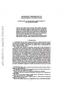
Proof. By induction. Consider m = 1. In this case it is clear, that there is only one regular graph 0 → 1 and Proposition 2.11 holds. Assume, that Proposition 2.11 holds for all m < m0 . Consider the path i and a corresponding graph Gi (see fig.1). This path has m0 + 1 distinct indices and 1

···

m0 − 1 m0

0

2m0 − 1

···

m0 + 1

Fig 1. The path i. Vertices, that correspond to equal indices, are connected via dotted lines.

it has 2m0 at all. It follows that there exist at least 2 one-element vertices of Gi . Let these one-element vertices be {s} and {t}. Consider the imsart-generic ver. 2009/08/13 file: matrix_power_mom.tex date: February 24, 2010


11

pair (it−1 , it )ε (t). It must have an equal pair, but it is not equal to any other index. It means, that (it−1 , it )ε(t−1) = (it , it+1 )ε(t) . It follows, that ε(t − 1) 6= ε(t). There are exactly two possibilities for this: t = m0 or t = 0. Assume without loss of generality that s = 0 and t = m0 . Therefore im0 −1 = im0 +1 (notice, that (m0 − 1) + (m0 + 1) = 2m0 ). Define (m0 − 1, 1)path j as follows: jk := ik if k ∈ {0, . . . , m0 − 2}, jm0 −1 := im0 −1 = im0 +1 , jk := ik+2 if k ∈ {m0 , . . . , 2(m0 − 1) − 1}. (See fig.2) The path j is the 1

··· m0 − 1 m0 + 1

0 2m0 − 1

m0

···

Fig 2. The path j is a (m0 − 1, 1)-path

(m0 −1, 1)-regular path. There is only one such path by inductive hypothesis and (ik = il ) ⇔ (jk = jl−2 ) ⇔ (k + (l − 2) = 2(m0 − 1)) ⇔ (k + l = 2m0 ). Definition 2.12. Notice, that the vertex of a regular graph has two outgoing edges iff the corresponding index has the form i2mk (because it should be (ij , ij+1 )ε(j) = (ij , ij+1 ) and (ij−1 , ij )ε(j−1) = (ij , ij−1 ) and it happens if and only if j = 2mk). The distance between such vertex and vertex V is called a type of vertex V. The type of index ij is the type of a vertex V such that j ∈ V. It is clear, that index ij has type j (mod 2m) if j (mod 2m) ∈ {0, . . . , m−1} or type −j (mod 2m) in the other case. There are m + 1 types of vertices. Note that only indices of the same type can be equal (this is proved in the case p = 1 in Proposition 2.11 and it will be proved for other cases below). Consider a collection of (m, pk )-regular paths (i0 , i1 , . . . , im ) (such that Pm k=0 pk = p−1) and collection of corresponding regular graphs (G0 , G1 , . . . , Gm ). Sum of path’s lengths is 2m(p − 1). We indicate the recipe how to obtain the (m, p)-regular graph from these collections. We take an (m, 1)-regular graph and attach to its vertices the graphs from the collection in the following way: the graph G0 is attached to vertex of type 0, the graph G1 is attached to vertex of type 1, . . . , the graph Pk Gm to the vertex of type m. For a more detailed argument we denote i=0 pi by Pk (Pm = p − 1) and the indices of (k) the kth path ik by ij . The resulting (m, p)-regular graph is denoted by Gj . imsart-generic ver. 2009/08/13 file: matrix_power_mom.tex date: February 24, 2010


12

Define the map ∆ : ∆(i0 , i1 , . . . , im ) = j as follows (0)

(0)

(0)

j0 := i0 , j1 = i1 , . . . , j2mP0 −1 := i2mp0 −1 , j2mP0 := j0 ; (1) (1) (1) j2mP0 +1 := i1 , . . . , j2mP1 −1 := i2mp1 −1 , j2mP1 := i0 , j2mP1 +1 := j2mP0 +1 ; (2)

(2)

(2)

(2)

j2mP1 +2 := i2 , . . . , j2mP2 −1 := i2mp2 −1 , j2mP2 := i0 , j2mP2 +1 := i1 , j2mP2 +2 := j2mP1 +2 ; ... (m) (m) (m) j2mPm−1 +m := im , . . . , j2m(p−1)−1 := i2mpm −1 , j2m(p−1) := i0 , j2mp−m+1 := j2mPm−1 +m−1 , . . . , j2mp−k := j2mPk +k , . . . , j2mp−1 := j2mP1 +1 . (2.22) e e Let ∆ is the corresponding map ∆(G0 , G1 , . . . , Gm ) = Gj . Graphically the constructon (2.22) looks as follows: (fig. 3). G0

0 2mP0

G1

G...

2mP0 + 1 2mP1 + 1

···

Gm−1

2mPm−1 + +m − 1, 2mp − m + 1

Gm

2mPm − m 2mp − m

Fig 3. The regular graph Gj , obtained from the collection of (m, pi )-regular graphs (G0 , G1 , . . . , Gm )

Example. For example, we consider for m = 2 the collection of (2, pk )regular graphs (G2,2 , G2,0 , G2,1 ) (see fig. 4) and we obtain from it a (2, 4)regular graph G2,4 (see fig.5). Proposition 2.13. Using the above construction we get an (m, p)-regular graph. Proof. Indeed, the graph Gj has exactly mp edges and kr = 2 for all r = 1, 2, . . . , mp. Furthermore, there are exactly Pm mp+1 vertices (there is no newintroduced vertex and there are exactly i=0 (mpi + 1) = m(p−1)+m+1 = mp + 1 vertices of graphs Gk ). Note, that the map ∆ is the injection. Now we consider the arbitrary (m, p)-regular path i and try to construct



0

4

2

13

6

1,3,5,7

1

G2,2 G2,1

0

2

Fig 4. Graphs G2,2 and G2,1 . Graph Gm,0 is empty

4

2

12

1,3,5,7

6

11,13

0,8

9,15

10,14

Fig 5. The resulting graph G2,4

inverse map for ∆. Denote J0 := {j : ij = i0 }; Jk := {j : j 6= 2mp − k, ij = i2mp−k }, k ∈ {1, . . . , m − 1}; Jm := {j : ij = i2mp−m }; Jk := max(Jk ), Jk := min(Jk ).

(2.23)

We will prove that the sets Jk have some remarkable properties and after that it will be clear, how to obtain a collection of regular paths from one (big) regular path. Proposition 2.14. Jk is nonempty. Proof. Indeed, there is 0 ∈ J0 and 2mp − m ∈ Jm . If Jk is void with k ∈ {1, . . . , m − 1}, then the index i2mp−k has no equal indices in the path imsart-generic ver. 2009/08/13 file: matrix_power_mom.tex date: February 24, 2010


14

i. But in this case the pair (i2mp−k−1 , i2mp−k )− has no equivalent for the following reason. The index i2mp−k appears in (2mp − k, 2mp − k + 1)− and in (2mp − k − 1, 2mp − k)− only and they are not equivalent. But each edge in a regular path has equivalent one, a contradiction. Therefore the initial assumption that Jk is void must be false. Proposition 2.15. Jk (0 ≤ k ≤ m) are pairwise disjoint and if k < l then Jk < Jl (for all j ∈ Jk and for all i ∈ Jl the inequality j < i holds). T Proof. Indeed, if Jk Jl 6= ∅ then i2mp−k = i2mp−l . The edges of the path i have the same orientation on the section (2mp−k, 2mp−k−1)− , . . . , (2mp− l + 1, 2mp − l) and therefore the graph T Gi has a cycle. But a regular graph is a tree, a contradiction. Thus Jk Jl = ∅. We prove the second part of Proposition 2.15 for the case l = k+1 only (which is sufficient). Consider the edge (2mp − (k + 1), 2mp − k)− . It must be equivalent to an edge (t, t + 1)+ with some t ∈TJk and t + 1 ∈ Jk+1 . If there exists s ∈ Jk such that s > t then s > t + 1 (Jk Jk+1 = ∅). The edge (t, t + 1) is not equivalent to any edge in the section (t + 1, t + 2), . . . , (s − 1, s), because it has only one equivalent edge (2mp − (k + 1), 2mp − k)− . It follows that there are two different paths in the graph Gi which connect vertex U (such that t + 1 ∈ U ) and vertex V (such that s ∈ V and t ∈ V), that is there is a cycle in the the graph Gi , and hence there is a contradiction. Therefore t = max Jk = Jk . Similarly, t + 1 = Jk+1 . It follows, that Jk + 1 = Jk+1 and for allj ∈ Jk and for all i ∈ Jk+1 the inequality j < i holds. Proposition 2.16. For all k the difference (Jk − Jk ) is divisible by 2m. Proof. Denote (Jk − Jk ) (mod 2m) by dk . Notice, that (Jk − Jk ) is the number of edges in the path’s section (Jk , Jk + 1), . . . , (Jk − 1, Jk ). Notice, that the orientation of edges changes after every m steps. Edges of the form (iJk , iJk+1 )+ have the same orientation. It follows, that d0 ≤ m − 1, d1 ≤ m − 1, (d0 + 1 + d1 ) ≤ m − 1 (mod 2m) (and so (d0 + 1 + d1 ) ≤ m − 1, because 0 ≤ d0 + 1 + d1 ≤ 2m − 1), . .P . , 0 ≤ d0 + 1 + d1 + 1 + ... + dm−2 + 1 + dm−1 ≤ m − 1 (similarly), i.e. 0 ≤ m−1 k=0 dk + m − 1 ≤ m − 1. Therefore, dk = 0 for all k = 0, 1, . . . , m − 1. Consider all edges of the path i. There are m edges of the form (Jk , Jk+1 ), m edges of the form (2mp − k, 2mp − k + 1)− with some k = 1, 2, . . . , m and all the remaing ones are in sections of the form (Jk , Jk + 1), . . . , (Jk − 1, Jk ). There are 2mp edges in total. Therefore, Pm Pm k=0 (Jk −Jk )+m+m = 2mp and hence k=0 dk = 0 (mod 2m). It follows, that dm = 0 too.



15

Proposition 2.17. If Jk < t < Jk and Jl < s < Jl , then it 6= is . In other words, sections of the path i of the form (Jk , Jk + 1), . . . , (Jk − 1, Jk ) with k = 0, 1, . . . , m are disjoint. Proof. Without loss of generality we consider l > k. Assume that it = is . In this case the section (Jk , Jk + 1), . . . , (s − 1, s) contains the edge (Jk , Jk+1 ), and the section (t, t + 1), . . . , (Jk − 1, Jk ) does not contain it or its equivalent (2mp − k − 1, 2mp − k)− . Thus, there are two non-equal paths in the regular graph Gi which connected vertex U (such that Jk ∈ U ) and vertex V (such that s ∈ V and t ∈ V), that is there is a cycle in the the graph Gi . Therefore, the initial assumption must be false. Now we can describe the inverse map for ∆. Let pk := (Jk − Jk )/2m (pk is a nonnegative integer by Proposition 2.16). Furthermore, we have for sum Pm−1 (k) the k-th k=0 pk = p − 1 (see the proof of Proposition 2.16). Denote by j resulting path (it has a length 2mpk and if pk = 0 then jk is empty). Let (k)

jt

:= iJk +((t−k)

mod 2mpk )) ,

t ∈ {0, . . . , 2mpk − 1}, k ∈ {0, . . . , m}. (2.24)

Now one obtains the collection (G2,2 , G2,0 , G2,1 ) (see fig. 4) from the graph G2,4 (see fig.5) in the way described in (2.24).

Proposition 2.18. The collection of paths (j(0) , j(1) , . . . , j(m) ) (defined by (2.24)) is the collection of regular paths.

Proof. In fact, the path j(k) is almost the same as the section (Jk , Jk + 1), . . . , (Jk − 1, Jk ) of the regular path i . This section contains 2mpk edges. Each of these edges has an equivalent one in the same section by Proposition 2.17. Therefore this section contains exactly mpk +1 distinct indices because of connectivity and non-cyclicity. Hence the path j(k) is a regular path. S reg reg reg reg e is the bijection between Tm,p Thus, ∆ and Tm,p 0 × Tm,p1 × · · · × Tm,pm , reg where the union is taken over all p0 + p1 + · · · + pm = p − 1. Hence #Tm,p = (m) Mp and Lemma 2.10 is proved. Lemmas 2.9 and 2.10 show that the moments of the spectral distribution (m) converge to Mp . Thus Theorem 1.1 is proved. References [1] Z. D. Bai, Methodologies in spectral analysis of large-dimensional random matrices, a review, Statist. Sinica 9 (1999), no. 3, 611-677. imsart-generic ver. 2009/08/13 file: matrix_power_mom.tex date: February 24, 2010


16

[2] Banica, T. Belinschi, S. Capitaine, M. and Collins B. Free Bessel Laws Preprint. arXiv:0710.5931 [3] Carleman T. Les fonctions quasi-analytiques, Paris, 1926. [4] Gessel, Ira M.; Xin, Guoce The generating function of ternary trees and continued fractions. Electron. J. Combin. 13 (2006), no. 1. [5] Ronald L. Graham, Donald E. Knuth, Oren Patashnik, Concrete Mathematics: A Foundation for Computer Science [6] Marchenko and V., Pastur, L. The eigenvalue distribution in some ensembles of random matrices. Math.USSR Sbornik, 1 (1967), 457-483 [7] W. Mlotkowski, Fuss–Catalan numbers in noncommutative probability, preprint. [8] A. Nica, R. Speicher, Lectures on the Combinatorics of Free Probability, Cambridge University Press, 2006 [9] F. Oravecz, On the powers of Voiculescus circular element, Studia Math. 145 (2001) [10] Wigner, E. On the distribution of the roots of certain symmetric matrices. Ann. of Math.67 (1958), 325–327.


Asymptotic distribution of singular values of powers of ... - CiteSeerX

Asymptotic distribution of singular values of powers of ... - CiteSeerX

Suggest Documents