Asymptotic Limits and Structure of the Pion Form Factor

arXiv:hep-ph/9611418v2 26 Nov 1996

Asymptotic Limits and Structure of the Pion Form Factor John F. Donoghue and Euy Soo Na Department of Physics and Astronomy University of Massachusetts Amherst, MA 01003 U.S.A. Abstract We use dispersive techniques to address the behavior of the pion form factor as Q2 → ∞ and Q2 → 0. We perform the matching with the constraints of perturbative QCD and chiral perturbation theory in the high energy and low energy limits, leading to four sum rules. We present a version of the dispersive input which is consistent with the data and with all theoretical constraints. The results indicate that the asymptotic perturbative QCD limit is approached relatively slowly, and give a model independent determination of low energy chiral parameters.

UMHEP-435; hep-ph/9611418 0

We are fortunate to have the rigorous techniques of perturbative QCD[1] and chiral perturbation theory[2] describing the high and low energy domains of the strong interactions respectively. The only comparatively rigorous techniques that apply to the intermediate energy region are lattice simulations[3] and dispersion relations[4]. Dispersive techniques are increasingly being combined with the other theoretical methods in order to provide as much control as possible throughout all energy regions. The simpliest cases are the two point functions of vector and axial vector currents[5],which are associated with the Weinberg sum rules[6] and other related sum rules. The next simpliest example is the three point function of the pion electromagnetic form factor. The purpose of this paper is to discuss the dispersive treatment of the pion form factor. We apply chiral constraints at low energy and incorporate the behavior of perturbative QCD at the highest energies. This leads to four sum rules, two of which are reasonably obvious and two which are new. In addition the dispersive treatment allows us to address the question of how fast the form factor approaches the asymptotic QCD behavior[7]. The form factor is defined by hπ + | Jµem | π + i = fπ (q 2 )(p + p′ )µ

(1)

with qµ = (p′ − p)µ In its twice subtracted form, the dispersion relation for the pion form factor reads q 4 ∞ ds Imfπ (s) fπ (q ) = 1 + Kq + (2) π 4m2π s2 s − q 2 − iǫ Our results are independent of the number of subtractions, but this form is most useful in presenting our techniques. We have imposed the normalization constant fπ (0) = 1, and the constant K is a subtraction constant to be determined below. At the high energy end, perturbative QCD tells us that the asymptotic behavior of the pion formfactor[7], with Q2 = −q 2 , is 2

fπ (Q2 ) = 16π

Z

2

αs (Q2 )Fπ2 64π 2 Fπ2 = 2 Q2 9 Q2 ln Q Λ2

with Fπ = 93MeV .

1

(3)

The fact that this decreases faster than 1/Q2 implies three sum rules when combined with Eq 2. The fact that there is no term proportional to Q2 as Q2 → ∞ implies a sum rule for the subtraction constant 1 K= π

Z

ds Imfπ (s) s2

∞

4m2π

(4)

Corresponding, there is no constant term as Q2 → ∞, requires a sum rule which can be found by Taylor expanding the denominator at large Q2 , yielding 1=

1 π

Z

∞

4m2π

ds Imfπ (s) s

(5)

Finally, the lack of a 1/Q2 term in the asymptotic region implies that 1Z∞ dsImfπ (s) (6) 0= π 4m2π These sum rules are contingent on the convergence of the integrals. This is especially relevant for the last one, but we will see that the integral is just barely convergent. At the low energy end, the pion form factor has been calculated to two loops in chiral perturbation theory. The result is fπ (q 2 ) = 1 +

2L¯9 2 q + cV q 4 + O(q 6) Fπ2

(7)

with L¯9 cV

m2π f¯1 m2π 1 ln + 1 + = − 192π 2 µ2 16π 2 Fπ2 ( ) 1 f¯2 1 = + 16π 2 Fπ2 60m2π 16π 2 Fπ2 !

(r) L9 (µ)

(8)

(r) In this expression, the parameters L9 (µ) and cV , f¯1 , f¯2 are renormalized pa(r) rameters from the E 4 and E 6 chiral Lagrangians, respectively. L9 (µ) can in principle be in other reactions, although it is most common to extract it from (r) this form factor. One give a dispersion sum rule for L9 (µ) by expanding the (r) chiral result around q 2 = 0 to find that L9 (µ) is related to the subtraction constant K defined above. The precise relation is

2

(r)

2L¯9 2L9 (µ) 1 m2π K= 2 = − ln +1 Fπ Fπ2 96π 2 Fπ2 µ2

!

(9)

Here and in what follows we drop reference to the chiral constant f¯1 since its effect is so small due to the factor of m2π multiplying it in Eq. 8. Note that relation for L¯9 is independent of the arbitrary scale µ, as the dependence of (r) L9 (µ) on µ is compensated by the explicit µ behavior displayed above. This exercise can be repeated to find the term at order Q4 , both in the dispersion relation and in the chiral expansion. The result is 1 cV = 16π 2 Fπ2

(

f¯2 1 + 60m2π 16π 2 Fπ2

)

1 = π

Z

∞

4m2π

ds Imfπ (s) s3

(10)

For completeness, let us briefly describe how these sum rules would be derived using an unsubtracted dispersion relation, 1 ∞ Imf (s) (11) ds π 0 s − q 2 − iǫ In this case, the sum rules of Eq. 5, 9, 10 all follows from Taylor expanding around q 2 = 0, while Eq. 6 follows from the q 2 → ∞ limit. Dispersion relations connect the high and low energy limits by providing constraints on the whole analytic functions. It is interesting that a given sum rule may follow from constraints on the high energy end in one derivation yet emerge in the low limit in another approach. We now turn to the construction of a representation of Imfπ (s) which is consistent with both the data and with theoretical constraints. The easiest step is at low energy, where chiral symmetry requires the structure[8] fπ (q 2 ) =

Z

2

s(1 − 4ms π )3/2 Imfπ (s) = θ(s − 4m2π ) + O(s2 ) 96π 2 Fπ2

(12)

In the intermediate energy region, we have data on both the real and imaginary parts of fπ (s). There is nothing surprising here, the physics is just that of the rho resonance. We take Imfπ (s) from a fit to the data in Ref[9]. Matching with the low energy limit is simple, as the resulting function is easily adjusted to approach Eq. 12 as s → 0. 3

For the high energy end, we need to choose an asymptotic form for Imfπ (s) which yields Eq. 3 when inserted in a dispersion relation. To see that this is the appropriate procedure, we consider dividing the dispersive integral into two pieces, with the transition part s¯ being large enough that above s = s¯ we are in asymptotic high energy behavior for Imfπ (s) 1 fπ (q ) = π 2

Z

0

s¯

Imf (s) 1 + ds s + Q2 π

Z

∞

s¯

ds

Imf (s) s + Q2

(13)

In the first integral the integrand is finite and the range is finite so that the result is analytic in 1/Q2 around Q2 → ∞. As a consequence, the logarithm in the QCD form for the asymptotic limit cannot be reproduced from the first integral, and must come from the s → ∞ behavior of Imfπ (s) in the second integral. The form of the imaginary part which guarantees the proper asymptotic limit is Imfπ (s) = −

1 64π 3 2 2 9 Q ln2 Q Λ2

(14)

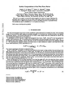
This form also allows the high energy sum rule Eq. 6 to converge. A final step is the matching between the intermediate and high energy forms of Imfπ (s). In order to help with this we impose the high energy sum rule Eq. 6 and the normalization integral Eq. 5. For these to be satisfied, the negative values of Imfπ (s) obtained from the asymptotic form at large s must extend to fairly low energies in order to be able to cancel the known positive contribution effects of the rho. This is a powerful constraint. There is certainly some ambiguity in the precise form in the matching region, but we have found a relatively simple solution. This is depicted in Fig. 1, showing a smooth matching slightly above 1 GeV . If we use this form for Imfπ (s) in a dispersion relation, we clearly have no predictive power in the intermediate energy region where our method is data-driven. The predictions come from the approaches to the asymptotic regions. Within a dispersive framework the transitions to the low energy and high energy limits are both determined largely by the numerically important intermediate energy region. Our results are presented graphically in Fig. 2. On the low energy side the structure of the real part of the form factor is governed by the low energy constraints of Eq. 9,10. These are predicted by the dispersion relations to have the form 4

(r) L9 (µ)

=

cV f¯2

= = =

m2π Fπ2 1 ln + 1 + 192π 2 µ2 2π 0.0074 4.1GeV −4 6.6 !

Z

∞

4m2π

ds Imfπ (s) s2

(15)

(r)

using µ = mη . The result for L9 agrees with the standard result, derived from the real part of the form factor. This is just a consistency condition for the dispersion relation. Of greater conceptional interest is the way that the dispersion method embodies the underlying physics of vector meson dominance(VMD), and the way that it resolves the issue of the scale dependence of the chiral coefficients in VMD[10]. Vector dominance is motivated by a narrow width approximation to the dispersion integral Imfπ (s) = πm2ρ δ(s − m2ρ )

(16)

Ecker, Pich and de Rafael argued that VMD determines the chiral coefficients at the scale µ2 = m2ρ . The dispersive approach provides a different answer (r) — VMD determines not simply the chiral coefficient L9 (µ) but rather the scale independent combination of the coefficient plus a specific combination of chiral logs, i.e. L¯9 in Eq. 9. On the high energy side, we see from Fig. 2 that the asymptotic QCD limit is approached rather slowly. In a dispersive framework this is due to the large contributions of the soft physics region, most notably the rho resonance, which continues to be more important in the dispersion integral than the somewhat small perturbative contribution. This result is consistent with quark model calculations[11], but is far less model dependent. The techniques of dispersion relations provide a partial bridge between the low energy techniques of chiral perturbation theory and the high energy techniques of QCD. The simplest exploration of these methods involve two point functions. The present work involves a three point function and hence is a step towards the consideration of yet more difficult matrix elements such as the nonleptonic amplitudes responsible for electromagnetic mass difference[12] or weak decays. References. 1) For a recent survey, see QCD - 20 Years Later, ed by P.M. Zerwas and 5

H.A. Kastrup (World Scientific, Singapore, 1993). 2) e.g. see J. F. Donoghue, E. Golowich and B. R. Holstein, Dynamics of the Standard Model, (Cambridge University Press, Cambridge, 1992). 3) A recent review is in Proc. XIV Intl. Conf. on Lattice Physics, (Elsevier Press, Amsterdam, 1996). 4)J. F. Donoghue, in Chiral Dynamics of Hadrons and Nuclei, ed by D.P. Min and M. Rho (Seoul National University Press, Seoul, 1995), p87 (hepph/9506205) and hep-ph/9607351. R. Kronig, J. Op. Soc. Am. 12, 547 (1926); H. A. Kramers, Atti Cong. Int. Fisici Como (1927). G. Barton, Dispersion Techniques in Field Theory, (Benjamin, NY, 1965). 5)J. Gasser and H. Leutwyler, Nucl. Phys. B250, 465 (1985). J. F. Donoghue and E. Golowich, Phys. Rev. D49, 1513 (1994). 6) S. Weinberg, Phys. Rev. Lett. 17, 616 (1966). T. Das, V. Mathur, and S. Okubo, Phys. Rev. Lett. 19, 859 (1967). T. Das, G. S. Guralnik, V. S. Mathur, F. E. Low, and J. E. Young, Phys. Rev. Lett. 18, 759 (1967). J. F. Donoghue and E. Golowich, Phys. Lett. 315, 406 (1993). J. F. Donoghue and E. Golowich, Ref 5. 7)S. J. Brodsky and G. P. Lepage, Phys. Rev.D22, 2150 (1980). A. Duncan and A. Mueller Phys. Rev. D21, 1636 (1980). 8)J. Gasser and H. Leutwyler, Ref 5. J. Gasser and U. G. Meissner, Nucl Phys. B357, 90 (1991). 9) A. Bericha, G. Lopez Castro, and J. Pestieau, Phys. Rev. D53, 4089 (1996). 10) J. F. Donoghue, C. Ramirez and G. Valencia, Phys. Rev. D39, 1947 (1988), G. Ecker, J. Gasser, A. Pich and E. de Rafael, Nucl. Phys. B321, 311 (1989). 11) N. Isgur and C. Llewellyn-Smith, Phys. Rev. Lett. 52, 1080 (1988), Nucl. Phys. B317, 526 (1989). L. S. Kisslinger and S. W. Wang, hep-ph/9403261 . 12) J. F. Donoghue and A. Perez, hep-ph/9611331, J. Bijnens and J. Prades, hep-ph/9610360.

6

Figure Captions Fig. 1. Fit to the imaginary part of the pion form factor satisfying the consistency constraints described in the text. Fig. 2. The real part of the pion form factor at large Q2 . The dashed line indicates the asymptotic prediction of perturbative QCD with Λ = 0.3GeV .

7