Asymptotic Normality of Linear Multiuser Receiver ... - Semantic Scholar

IEEE TRANSACTIONS ON INFORMATION THEORY, VOL. 48, NO. 12, DECEMBER 2002

1

Asymptotic Normality of Linear Multiuser Receiver Outputs Dongning Guo, Sergio Verd´ u, and Lars K. Rasmussen a short-code system, the system size has to be much larger in order for the error in this approximation to normality to be negligible. Nevertheless, the distribution of the MAI in a matched filter output is shown to converge to a Gaussian law in the sense of divergence by Verd´ u and Shamai [11]. In fact, [11] is one of the first to prove asymptotic normality for an output distribution conditioned on the spreading sequences. Moreover, Poor and Verd´ u [12] showed that the distribution of the output MAI of the MMSE receiver in a short-code system often has no noticeable difference to a Gaussian law. Recently, it was proved rigorously by Zhang et al. that the MAI in the MMSE receiver output is asymptotically Gaussian [13]. Normality is also established for linear blind multiuser receivers [14]. Index Terms: Code-division multiple access, multiuser These normality results allow the large-system probabildetection, multiple access interference, central limit theo- ity of error of these receivers to be quantified by a sinrem, multiuser efficiency, signal-to-interference ratio. gle Q-function of the square root of the output signal-tointerference ratio (SIR). It also implies that error-control I. Introduction codes for Gaussian channels are asymptotically optimal if Linear multiuser receivers for multiple access channels autonomous single-user decoding is to be used. As a result, have been studied extensively during the last two decades the receiver and the decoder can be designed and optimized due to their performance capabilities and analytical tractabil- separately. ity [1]. A linear receiver provides a soft output that can be The normality property of all the above mentioned reeither hard limited for decision-making or treated as soft re- ceivers is not accidental. Indeed, this is a result of the liability information for further processing such as in coded central limit theorem due to the fact that the MAI is a transmission [2], [3]. The conventional matched filter, the sum of contributions from a large number of users. In this decorrelator and the minimum mean square error (MMSE) paper, we extend the normality principle to a much wider receiver are among the earliest and most well-known linear family of linear receivers, which is defined as a set of mareceivers. More recently, linear interference cancelers have trix filters each of which shares the same eigenvectors as also been analyzed [4], [5], [6], [7], [8], [9]. those of the channel correlation matrix and takes eigenvalThe performance, in particular, the uncoded bit-error- ues given by a function of the eigenvalues of the correlation rate (BER) of a linear receiver, depends on the cumula- matrix. Immediately, this family includes the conventional tive distribution of the multiple access interference (MAI), receiver, the decorrelator, and the MMSE receiver. Also, it which is in general a discrete distribution. For all but the includes a subset of matrix filters described by polynomial decorrelator, the BER is given as a sum of an exponen- expansion of the correlation matrix, called polynomial retial number of Gaussian error functions (Q-functions1 ), the ceivers [15], which corresponds exactly to the set of linear evaluation of which is infeasible for even moderately sized multistage parallel interference cancelers [16]. systems. Our results are asymptotic in nature, namely, they are To circumvent this difficulty, a Gaussian approximation large-system limits where the number of users and the of the MAI is often used. Weber et al. [10] were among the spreading factor both tend to infinity with a fixed ratio. earliest to model interfering users’ signals as white Gaus- Recent work in [17], [18], [11], [13], [19] shows that this apsian noise. Since then a large amount of work has been proach can average out the dependence on specific spreaddedicated to the justification of various normality approx- ing sequences and result in simple expressions for system imations. For a long-code system, the MAI embedded in performance. Moreover, asymptotic results provide good the output of the matched filter for each user can be well approximations for moderately sized systems in many cases approximated by a Gaussian random variable [1], [11]. For of practical interest. Our results can be summarized as follows. Assuming This work was supported in parts by the National Science Founrandom spreading sequences, the output decision statistic dation under grant no. CCR0074277 and by the Swedish Research of the family of linear receivers for each user is asymptotCouncil for Engineering Sciences under grant no. 217-1997-538. R ∞ −t2 /2 1 Q(x) = √1 ically Gaussian in distribution conditioned on one’s own e dt 2π x Abstract— This paper proves large-system asymptotic normality of the output of a family of linear multiuser receivers that can be arbitrarily well approximated by polynomial receivers. This family of receivers encompasses the singleuser matched filter, the decorrelator, the MMSE receiver, the parallel interference cancelers, and many other linear receivers of interest. Both with and without the assumption of perfect power control, we show that the output decision statistic for each user converges to a Gaussian random variable in distribution as the number of users and the spreading factor both tend to infinity with their ratio fixed. Analysis reveals that the distribution conditioned on almost all spreading sequences converges to the same distribution, which is also the unconditional distribution. This normality principle allows the system performance, e.g., the multiuser efficiency, to be completely determined by the output signalto-interference ratio for large linear systems.

IEEE TRANSACTIONS ON INFORMATION THEORY, VOL. 48, NO. 12, DECEMBER 2002

transmitted symbol. Moreover, the asymptotic output distribution of a receiver in this family is the same conditioned on almost all possible spreading sequences, which is also the asymptotic unconditional distribution. The normality principle holds for very general scenarios. The spreading sequences are not limited to binary sequences and the received energies of the users can be different. Our results follow the work of Zhang et al. [13], where asymptotic normality was concluded for the MMSE receiver only. Besides making use of some of the same mathematical tools as in [13], our proof is quite different. We tackle the problem by starting from polynomial receivers. We show that the output decision statistic of every polynomial receiver is asymptotically Gaussian in distribution. We then generalize the normality principle to a large family of receivers that can be approximated arbitrarily by polynomial receivers. This paper is organized as follows. Section II introduces the system model and notation. Polynomial receivers are studied under the perfect power control assumption in Section III. The normality principle is generalized to a family of receivers in Section IV. Arbitrary energy distribution is considered in Section V. Results on some popular receivers are summarized in Section VI. Some numerical examples are given in Section VII. II. System Model A. CDMA Uplink Channels We assume a symbol-synchronous CDMA system depicted in Fig. 1 where each user’s spreading sequence is independently and randomly chosen. For the purpose of large-system analysis, we consider first a K-user system with a spreading factor of N = N (K) and then let K and N go to infinity with their ratio converging to a non-negative number β, i.e., lim

K→∞

K = β. N (K)

converge as K → ∞ to a distribution FP , called the energy distribution, which has finite moments of any order. Let {¯ snk | n = 1, 2, · · · , k = 1, 2, · · · } be an infinite array of real-valued independent identically distributed (i.i.d.) random chips. For convenience we assume that the distribution of the chips has unit-variance and finite higher order moments, and is symmetric, i.e., −¯ snk follows the same distribution as s¯nk . Consider a K-user system. The spreading sequence of user k is given as an N -dimensional (K) vector, ¯sk = √1N [¯ s1k , s¯2k , · · · , s¯N k ]>. We define the unnormalized spreading sequence of user k to be (K)

sk

p 1 (K) = √ [s1k , s2k , · · · , sN k ]> = Pk ¯sk . N

(2)

k=1

In Section III and IV, we study the simplest perfect power control case, where the received energies are equal from all users, i.e., Pk = 1 for k = 1, . . . , K. In Section V, we allow the received energies to be different. We assume, however, that the empirical distributions of {P1 , . . . , PK } 2 The SIR is defined as the energy ratio of the useful signal to the noise in the output. In contrast, the signal-to-noise ratio (SNR) of user k is usually defined as the ratio of the input energy and singlesided noise spectral density Pk /(2σ 2 ).

(3)

We also define the unnormalized correlation matrix R(K) as a K × K random matrix with its element on the k th row and the j th column as the crosscorrelation of user k and user j’s unnormalized spreading sequences, p N N h i Pk Pj X 1 X R(K) = s>k sj = snk snj = s¯nk s¯nj . N n=1 N kj n=1 (4) Note that we label the correlation matrix with its corresponding system dimension (the number of users). In fact, every variable pertaining to a K-user system has K as its corresponding dimension. For notational convenience, we will often omit the index (K) when the dimension is understood from the context. For instance, R(K) is simplified to R. Let {dk | k = 1, 2, · · · } be a sequence of independent random antipodal modulated symbols taking the value of +1 and −1 equally likely. For a K-user system, let d = [d1 , · · · , dK ]> be the vector of transmitted symbols. A set of sufficient decision statistics is obtained by matched filtering using all user’s unnormalized spreading sequences3

(1)

Let {Pk | k = 1, 2, . . . } be a deterministic sequence consisting of the received energies per symbol of all users. The signal-to-interference ratio2 of user k in absence of interfering users is therefore Pσk2 . By absorbing a common factor into the noise level, we can assume without loss of generality for a K-user system K 1 X Pk = 1. K

2

yMF = Rd + n

(5)

where the correlation matrix R is determined by (4), and n is a zero-mean Gaussian noise vector with covariance matrix σ 2 R, where σ 2 is the noise sample variance. B. Linear Receivers A linear receiver assumes knowledge of the spreading sequences, the received energies, as well as the noise variance and makes use of this information in detection. Mathematically, it is a K × K matrix filter G, dependent on R and σ 2 , applied to the matched-filter output. It outputs a vector of decision statistics expressed as y

= G · yMF = G · (Rd + n) = (GR) · d + z

(6) (7) (8)

where z = Gn is a zero-mean Gaussian random vector with covariance matrix σ 2 GRG>. We denote GR by H 3 This is in contrast to matched filtering using normalized spreading sequences as in [1].

IEEE TRANSACTIONS ON INFORMATION THEORY, VOL. 48, NO. 12, DECEMBER 2002


  

     


  

      

>> >

" #%$& '  

 ! (



)+*-, /.0  :;2  *   132545,  < 6798   25= 

 

   



    >> >


  

       ) @ ? 254 BA ,C*-,C2 @A

3

 )+D45,C2FE04 *  AGA H. * 0 4

   

I * AC JA ,C*-,C2 @

Fig. 1. Discrete time system model.

throughout the paper for notational simplicity. Thus, we have a simple linear system expressed as y = H · d + z.

(9)

An advantage of linear receivers is that they can be implemented in a decentralized fashion [1]. Independent single-user decoding is conducted based on the decision statistic sequence produced by the individual linear receiver. From an individual user’s point of view, the multiaccess channel collapses to a single-user channel by treating the MAI as noise. The input-to-output characteristic of such a single-user channel is determined by the distribution of the output decision statistic conditioned on the transmitted symbol. Without loss of generality, we consider user 1. As far as the performance is concerned, we can assume that user 1 always transmits +1.4 User 1’s decision statistic is a scalar y1 = H11 +

K X

H1k dk + z1

(10)

k=2

where Hkj , like [H]kj , denotes the element of H on the k th row and the j th column. Clearly, this decision statistic consists of the transmitted symbol (d1 = 1) scaled by H11 , the multiaccess interference aggregated from all the other users, and a Gaussian noise term. We can interpret the randomness of the decision statistic in two different ways which correspond to short-code and long-code systems respectively. In a short-code system, the spreading sequences are randomly picked at the beginning of transmission and remain the same for every transmitted symbol. For each channel use, the randomness in y1 includes that of the transmitted symbols and that of the noise. The performance, e.g. the uncoded probability of error, can be easily obtained once we have the distribution of y1 conditioned on the spreading sequence. In a longcode system, the spreading sequences are randomly and independently chosen symbol-by-symbol. The randomness of y1 then also includes the randomness of the crosscorrelations reflected in matrix H. The expected performance, 4 Accordingly, all distributions we will be considering are implicitly conditioned on d1 = 1.

for instance the uncoded error probability averaged over all spreading sequences, is now better characterized by the unconditional distribution of y1 . In this paper we address both the conditional distribution and the unconditional distribution as the system size increases without bound. The resulting distributions turn out to be the same for all but a negligible set of spreading sequences. C. A Family of Linear Receivers Note that R is symmetric. It has an eigen-decomposition as R = UΛU>

(11)

where U is unitary and Λ = diag(λ1 , · · · , λK ) is a diagonal matrix consisting of the eigenvalues of R, which are all nonnegative random variables dependent on R. We limit our study to receivers taking the form of G = U · diag(g(λ1 ), · · · , g(λK )) · U>

(12)

for some real continuous function g, and refer to them as the family of linear receivers throughout this paper. With slight abuse of notation we denote the right hand side of (12) by g(R). Note that g(R) is symmetric and shares the same eigenvectors with R, and the eigenvalues of g(R) are given by the function g evaluated at the eigenvalues of R. The family of receivers defined in the above represents a subset of linear receivers. It does not include successive interference cancelers, which, unlike (12), treat users unequally. Neither does it include the optimum linear detector in the sense of BER or asymptotic multiuser efficiency [1, Page 288]. Nonetheless, a wide spectrum of linear receivers belong to this family. In particular, if the function g degenerates to a constant 1, the receiver G is reduced to the single-user matched filter. If g is a polynomial, G becomes a polynomial receiver (or, equivalently, a parallel interference canceler [16]). If we let ( 1 if λ > 0, (13) g(λ) = λ 0 if λ = 0,

IEEE TRANSACTIONS ON INFORMATION THEORY, VOL. 48, NO. 12, DECEMBER 2002

the resulting G is the decorrelator. If we let g(λ) = (λ + σ 2 )−1 , G becomes the MMSE receiver. Let us include the dimension index for the rest of this section to make it clear what we mean by a linear receiver in the large-system analysis. Alinear receiver here refers ∞ to a sequence of matrix filters G(K) K=1 , each G(K) a function of R(K) , for which the vector of output decision statistics is expressed as y

(K)

=G

(K)

·

(K) yMF .

4

III. Polynomial Receivers Under Perfect Power Control In this section, we study a subset of linear receivers, namely, the set of polynomial receivers, special cases of which have been considered in [15], [5], [23]. A polynomial receiver G is of the form G=

xi Ri−1

(22)

i=1

(14)

In particular, a linear receiver in the family of our interest is defined as a sequence of receivers specified by a function g, i.e., for K = 1, 2, . . . ,   >  (K) (K) G(K) = U(K) · diag g(λ1 ), · · · , g(λK ) · U(K)

m X

where m is an integer, and the weights xi are arbitrary deterministic real numbers. G can be expressed as a member of the family of receivers defined by (12) if we let g be a polynomial g(λ) =

(15)

m X

xi λi−1 .

(23)

i=1

where

We study the marginal probabilistic law of the decision (K) statistic y(K) , i.e., the distribution of y1 , as K goes to infinity.

We study the output distribution of the polynomial receiver G in both the conditional case and the unconditional case. In this section, we also limit ourselves to the equal-energy case, i.e., Pk = 1, k = 1, . . . , K, for which we obtain simple expressions for the limiting distribution. The results are extended to unequal-energy case in Section V.

D. Eigenvalue Distribution

A. Conditional Distribution

The normality results we will show in the following sections hinge on the intriguing fact that the limiting empirical distribution of the eigenvalues of a large random covariance matrix is deterministic. Denote the limit of the cumulative distribution of the eigenvalues of the random matrix R(K) by FΛ . It is dependent on the received energy distribution FP . In general, this distribution function does not have a closed-form solution. Its Stieltjes transform, defined as Z 1 m(z) = dFΛ (λ) (17) λ−z

Consider the MAI term in the decision statistic y1 in (10) where H is given. It is a sum of contributions from all interfering users. Due to the central limit theorem, its distribution becomes closer and closer to a Gaussian law as the system size increases without bound. Precisely, we have the following theorem. Theorem 1: The decision statistic (10) as a function of H, where the polynomial receiver is given as (22), converges to a Gaussian random variable in distribution with probability 1. The mean value corresponding to the limiting distribution is

  >  (K) (K) R(K) = U(K) · diag λ1 , · · · , λK · U(K) .

(16)

satisfies  Z m(z) = −z + β −1

−1 P dFP (P ) 1 + P m(z)

µ1 =

xi Mi

(24)

xi xj [Mi+j − Mi Mj + σ 2 Mi+j−1 ]

(25)

(18)

where FP is the energy distribution [20], [21]. In the equal-energy case, a closed-form solution exists [22]   Z λ 1 FΛ (λ) = max 0, 1 − · u(λ) + pβ (t) dt (19) β −∞

m X i=1

and the variance is σ12 =

m X m X i=1 j=1

where Mi is defined as where u(λ) is a unit step function, and   ( p Mi = lim E Ri 11 . (26) 1 (λ − λ )(λ − λ) if λ < λ < λ , K→∞ min max min max pβ (λ) = 2πβλ 0, otherwise, In the special case of perfect power control, Mi is equal to (20) the ith -order moment of the limiting eigenvalue distribution √ √ with λmin = (1 − β)2 and λmax = (1 + β)2 . An expres- given by (21). Note that surprisingly the mean and the variance are not sion for the moments of the eigenvalues has been developed dependent on R, since Mi is an average over all spreading in [22] sequences. Indeed, the theorem states that the asymptotic    i−1 conditional distribution is almost surely independent of the  i X 1 i i−1 E λ = βj . (21) spreading sequences. We develop a proof of the theorem j j j+1 j=0 starting from showing the existence of Mi .

IEEE TRANSACTIONS ON INFORMATION THEORY, VOL. 48, NO. 12, DECEMBER 2002

5

Lemma 1: Under perfect power control,   Mi = lim E Ri 11

has finite moments of any order. This allows us to have a clear picture of the probabilistic property of the elements (27) in Ri . By first subtracting its mean value (the off-diagonal K→∞ elements have zero-mean) each entry diminishes as K → exists and is given by (21).  i ∞. This vanishing rate is quite fast. In fact, if we amplify Proof: Under perfect power control, R kk ’s are it by √K, each entry converges to some random variable, identically distributed for all k. Hence the moments of which are the finite limits of the central moments of (35). K   1 X  i  A weaker boundedness result is sufficient √ for our E R kk (28) = E Ri 11  study,  K namely, the pth order central moment of K Ri 1k is k=1 bounded by some number for all K, due to its convergence. 1   i = E tr R (29) The following is immediate. K (K ) th Corollary 1: For every X  positive integer p, the p −order p 1 i i = E λk (30) central moment of R 1k is upper bounded by γK 2 for K all p and K where γ is a positive number independent of k=1  = E λi (31) K. Corollary 1 leads to the following almost sure converwhere λ is a randomly picked eigenvalue of Ri . Taking the gence.   large-system limit of both sides of (31), the left hand side Lemma 3: Ri 11 converges to Mi with probability 1 as is Mi and the right hand side is given by (21). K → ∞. We next present a simple fact that underlies all major Proof: Define results in this paper.     vK = Ri 11 − E Ri 11 . (36) Lemma 2: Let {ˆ snk | n = 1, 2, · · · , k = 1, 2, · · · } be an array of independent random variables each taking equally likely values of +1 and −1. Let n1 , · · · , ni ∈ {1, · · · , N } The system dimension (K) is explicit in vK . By Corollary 1, there exists γ > 0, and k1 , · · · , ki , ki+1 ∈ {1, · · · , K}. Then the product  4 γ sˆn1 k1 sˆn1 k2 sˆn2 k2 sˆn2 k3 · · · sˆni−1 ki−1 sˆni−1 ki sˆni ki sˆni ki+1 (32) E vK < 2 , ∀K. (37) K is a constant +1 if the indexes are such that all the indexed By the Markov Inequality [24], for every  > 0, sˆ variables appear in pairs; otherwise the product is a ran 4 dom variable taking the values of +1 and −1 equally likely. E vK (38) P (|vK | > ) ≤ 4 This Lemma holds trivially. For example, sˆ21 sˆ24 sˆ14 sˆ14 sˆ24 sˆ21 γ < . (39) consists of 3 pairs of identical binary variables and is equal 4K 2  2 2 2 to sˆ21 sˆ24 sˆ14 = +1. On the contrary, sˆ12 sˆ11 sˆ31 sˆ32 is a fair Clearly, coin toss of +1 and −1, and has a zero mean. Every entry in the matrix Ri is a highly structured weighted ∞ X sum of products of the form of (32), P (|vK | > ) < ∞. (40)  i K=1 R 1k =

K X

R1k2 Rk2 k3 · · · Rki k

(33)

k2 ,...,ki =1

=

1 Ni

K X

N X

k2 ,...,ki =1

n1 ,...,ni =1

sn1 1 sn1 k2 sn2 k2 sn2 k3 · · · sni−1 ki−1 sni−1 ki sni ki sni(34) k. Lemma 2, reinforced with combinatorial arguments, powerfully reveals the probabilistic behavior of individual elements in Ri . We have the following proposition, the proof of which is quite lengthy and relegated to Appendix I and II. Proposition 1: For every positive integer p, √and every  user index k, the pth -order central moment of K Ri 1k converges to a deterministic constant as K → ∞. As a consequence, the asymptotic distribution of √    
K Ri 1k − E Ri 1k (35)

By the Borell-Cantelli Lemma [25], vK converges to 0 with probability 1. Therefore,  i   R 11 = E Ri 11 + vK (41) converges with probability 1 to Mi by Lemma 1. The following is immediate from Lemma Pm 3.   Corollary 2: The coefficient H11 = i=1 xi Ri 11 conPm verges to i=1 xi Mi with probability 1. Also, we have the following lemma about the MAI term in (10). PK Lemma 4: The distribution of k=2 H1k dk , conditioned on the spreading sequences, converges to a Gaussian law with probability 1. To prove Lemma 4, we use the Lindeberg-Feller central limit theorem [26, page 448], which is restated here in a form convenient for this paper.

IEEE TRANSACTIONS ON INFORMATION THEORY, VOL. 48, NO. 12, DECEMBER 2002

6

Theorem 2 (Lindeberg-Feller) For each K, let {XK,1 , . . . , Since dk = ±1, and noting that XK,K } be independent zero-mean random variables with  x n , ∀ x, , n > 0, 1{x>} ≤ finite variance. Suppose that  K X  2 E XK,k → 1,

(42)

k=1

we have WK (H, ) =

and that the Lindeberg condition is satisfied, i.e., for all  > 0, K X  2 lim E XK,k · 1{|XK,k |>} = 0

K→∞

K→∞

(44) Condition (L4.1) holds for all H by independence of dk ’s. The sum in condition (L4.2) can be obtained as =

k=2

=

K X

2 H1k Hk1 − H11

k=1 2

2 [H ]11 − H11 .

(45) (46)

Notice that H2 =

m X m X

xi xj Ri+j .

(47)

i=1 j=1

The right hand side of (46) converges to m X m X i=1 j=1

xi xj Mi+j −

m X

!2 xi Mi

(48)

i=1

K o n X 2 E (H1k dk ) · 1{|H1k dk |>} H . k=2

P (WK (H, ) > δ) ≤ ≤

(51)

4 H1k 4

(52)

2 H1k ·

1 · E {WK (H, )} δ (K ) X 1 6 ·E H1k δ4

(53) (54)

k=2

= ≤

 6 K −1 · E H12 (55) 4 δ n o √ 1 · E ( KH12 )6 (56) 4 2 δ K

where (53) is by the Markov Inequality and (55) holds because the H1k ’s, k = 2, · √ · · , K, are identically √ distributed.   Pm Since every moment of KH1k = x K Ri 1k is i i=1 bounded due to Corollary 1, the probability P (WK (H, ) > δ) is bounded by some γK −2 which is summable over K. Analogously to Lemma 3, the Borell-Cantelli Lemma leads to lim WK (H, ) = 0 with probability 1,

K→∞

(57)

i.e., the Lindeberg condition (L4.3) is satisfied with probability 1. In all, conditions (L4.1-3) are satisfied with probability 1. Invoking Theorem 2, we obtain that conditioned on almost all spreading sequences, the MAI is asymptotically Gaussian. With the distribution of all three components of the decision statistic (10) known (the noise is trivially Gaussian), we can now prove its asymptotic normality. Proof: [Theorem 1] The first term on the right hand side of (10) converges with probability 1 to a deterministic value by Corollary 2. The MAI term is asymptotically Gaussian with probability 1 by Lemma 4. The noise is zero-mean Gaussian with variance  E z12 = [GRG]11 σ 2 , (58) which can be easily shown to converge to 2 ν∞ = σ2

with probability 1 by Corollary 2. To examine condition (L4.3) we define WK (H, ) =

2 H1k · 1{|H1k |>}

Hence for every δ > 0,

k=2

2 H1k

K X k=2

(43)

k=1

K o n X 2 E (H1k dk ) · 1{|H1k dk |>} H = 0, ∀ > 0.

K X

K X k=2

≤

where 1{·} is the indicator function which takes the value of 1 if the condition in the braces is satisfied and 0 otherPK wise. Then k=1 XK,k converges to a standard Gaussian random variable in distribution. Lemma 4 can be proved as follows. Proof: [Lemma 4] Assume that the spreading sequences are given so that H is determined. We study the set of random variables {H12 d2 , . . . , H1K dK } for each K and show that for almost all possible spreading sequence assignments, the conditions required by Theorem 2 are satisfied, namely, (L4.1) {H1k dk | k = 2, · · · , K} is a set of independent zeromean random variables; o n PK 2 (L4.2) E (H d ) 1k k H converges as K → ∞; and k=2 (L4.3) The Lindeberg condition lim

(50)

m X m X

xi xj Mi+j−1

(59)

i=1 j=1

(49)

with probability 1. Conditioned on the spreading sequences, the MAI and the noise are independent. The distribution of the decision statistic is therefore asymptotically Gaussian with mean value and variance given by (24) and (25) respectively.

IEEE TRANSACTIONS ON INFORMATION THEORY, VOL. 48, NO. 12, DECEMBER 2002

B. Unconditional Distribution

7

To verify (T3.3), we find, for every  > 0

It is also desirable to know the distribution of the deK n o X 2 cision statistic when the spreading sequences are allowed E (H1k dk ) · 1{|H1k dk |>} to vary symbol-by-symbol as in a long-code system. In k=2  2 every symbol interval, the MAI is a large sum of contri= (K − 1) · E H12 · 1{|H12 |>} (64) butions from individual interfering users, whose spreading  1 4 sequences are chosen independently from that of the desired (65) ≤ (K − 1) · 2 · E H12  user. It is expected that the MAI approaches a Gaussian n√ o 1 probability law in distribution as the number of users in≤ · E ( KH12 )4 (66) 2 K creases. The resulting distribution is trivially the same as → 0 (67) in the conditional case since the unconditional distribution is a mixture of the conditional ones, the limit of which are as K → ∞ by Corollary 1. PK all the same except for a negligible set in probabilistic sense With conditions (T3.1)–(T3.3) verified, the sum k=2 H1k dk by virtue of Theorem 1. Precisely, we have the following converges to a Gaussian law, with zero mean and a variance theorem. given by (48), following a dependent central limit theorem Theorem 3: The unconditional distribution of the decifor martingales in [27]. sion statistic given by (10), where the polynomial receiver Moreover, the noise converges trivially to a Gaussian is given as (22), converges to a Gaussian law with mean random variable in mean square sense. Note that both value and variance given by (24) and (25) respectively. the MAI and the noise are dependent on the spreading seProof: We present a direct proof similar to that of quences. Given the output noise variance, however, the the conditional case rather than citing Theorem 1. The noise and the MAI are mutually independent. Consider a proof reveals some dependence subtleties not present in slight modification of the decision statistic, where we inthe conditional case. Pm troduce a scalar multiplier to the noise term to remove First, H11 → i=1 xi Mi with probability 1 by Coroldependence, lary 2. PK Second, we need to show that the distribution of k=2 H1k dk K X ν∞ converges to a Gaussian law. This is not as simple as in the · z1 (68) y10 = H11 + H1k dk + p E {z12 } conditional case, since the H1k ’s are now dependent rank=2 dom variables. We resort to a more general central limit theorem in [27]. We show that the following 3 conditions where ν∞ is defined p in (59). The standard Gaussian random variable z / E {z12 } can be easily shown to be inde1 are satisfied. PK pendent of the spreading sequences and hence of the MAI. (T3.1) k=2 H1k dk is a martingale for every K; P 2  Since the multiplier converges to 1, (y10 − y1 ) converges to 0 K (T3.2) E converges as K → ∞; and in mean square sense, and hence y1 and y10 share the same k=2 H1k dk asymptotic distribution. (T3.3) The Lindeberg condition is satisfied, i.e., In all, the distribution of y1 is asymptotically Gaussian K with a mean value as that of the limit of the first term, and n o X 2 E (H1k dk ) · 1{|H1k dk |>} → 0, ∀ > 0. (60) a variance as the sum of the limits of those of the MAI and the noise. They are given in (24) and (25), respectively. k=2 For every K, and an arbitrary user index k > 1, the conditional expectation E {H1k dk |H12 d2 , · · · , H1 k−1 dk−1 } = 0

(61)

by independence of the data symbols. By definition, H1k PK is an absolutely fair sequence, and therefore k=2 H1k dk is a martingale [25, p. 209]. Hence (T3.1) is true. Also by the independence of the antipodal symbols,  !2  K K  X  X  2 E H1k dk = E H1k (62)   k=2 k=2   2 . (63) = E [H2 ]11 − E H11 The right hand side of (63) converges by Corollary 2. Thus we have (T3.2).

IV. Asymptotic Normality We have shown above that, under perfect power control, every polynomial receiver yields asymptotically Gaussian outputs. By the Weierstrass Theorem, the set of polynomials is dense in the space of continuous functions defined on a finite interval [28]. For this reason, we can show that every receiver of the form G = g(R) can be arbitrarily well approximated by a sequence of polynomial receivers. As a consequence its output is also asymptotically Gaussian in distribution. Formally, we have the following theorem. Theorem 4: Assume perfect power √control. √ For every
function g continuous on max2 (0, 1 − β), (1 + β)2 , the output decision statistic of any linear receiver G = g(R) defined in (12) is asymptotically Gaussian in distribution conditioned on almost all spreading sequences. The mean value corresponding to the limiting distribution is Z µg = g(λ) · λ dFΛ (λ) (69)

IEEE TRANSACTIONS ON INFORMATION THEORY, VOL. 48, NO. 12, DECEMBER 2002

and the variance is Z σg2 = g 2 (λ) · λ · (λ + σ 2 ) dFΛ (λ) − µ2g .

(70)

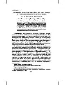
The following lemma is useful for proving Theorem 4. Lemma 5: Let G = g(R). For all  > 0, there exists a ˜ = g˜(R) such that the mean square polynomial receiver G difference of every user’s output decision statistic of G and ˜ is less than  for sufficiently large K for almost all spreadG ing sequences. Lemma 5, proved in Appendix III, establishes that a linear receiver can be arbitrarily well approximated by polynomial receivers in the large-system limit. The fact that the output of every polynomial receiver converges to a Gaussian random variable leads to the asymptotic normality of linear receiver outputs. The proof of Theorem 4 also requires the following n lemma. o (K) Lemma 6: Let Ym K = 1, 2, · · · , m = 1, 2, · · · be an  ∞ array of continuous random variables. Let Y (K) K=1 and {Ym }∞ m=1 be two sequences of random variables. Denote (K) the cumulative distribution functions of Ym , Y (K) and (K) Ym as Fm , F (K) and Fm respectively. Suppose that  2  (K) (K) − Ym = 0; and(71) (L6.1) lim lim E Y m→∞ K→∞ (K) (L6.2) lim Fm (a) − Fm (a) = 0, ∀a, m, (72)

8

Proof: [Theorem 4] For clarity, we explicitly label relevant variables with their corresponding system dimension. Take a sequence m → 0. For n eachom, by Lemma 5, (K) there exists a polynomial receiver Gm determined by a polynomial gm such that for sufficiently large K and almost all spreading sequences,  2  (K) (K) (73) E y1 − ym1 < m (K)

(K)

(K)

where y1 and ym1 are the output of G and Gm for user 1 respectively. (K) (K) (K) Let Y (K) = y1 and Ym = ym1 . Due to the presence (K) of noise, Ym are continuous random variables. Equation (73) implies (71). Also, by Theorem 1, for every m, (K) Ym converge as K → ∞ to some Gaussian random variable, defined as Ym . Hence (72) is satisfied. Note that a sequence of Gaussian distribution functions converge also to a Gaussian law. Invoking Lemma 6, we have that Y (K) converge in distribution to a Gaussian law. Equation (69) Pm is straightforward by noting that for gm (λ) = i=1 xi λi−1 , (m ) m X X xi Mi = E xi λi (74) i=1

i=1

= E {gm (λ) · λ} Z = gm (λ) · λdFΛ (λ).

(75) (76)

K→∞

Equation (70) can be obtained analogously. then both F (K) and Fm converge pointwise to the same distribution.

system size K → ∞ −−(1) −−−−− −−−−−(2) −−−−−−−−−− −−−−−−−−−−−−−− −−−−−−−→ (K)  Y1 · · · Y1 · · · → Y1  g1 Y1    (1) (2) (K) g2  Y2 · · · Y2 · · · → Y2   Y2    ..  .. .. .. ..    .  . . . .   (1) (2) (K) gm Ym Ym · · · Ym · · · → Ym  Gaussian ..    .. .. .. ..   .  . . . .      ↓  ↓ ↓ ↓ ↓     g(R) yY (1) Y (2) · · · Y (K) · · · → Y  Fig. 2. Convergence of output distributions.

The proof of Lemma 6 is in Appendix IV. The idea is illustrated in Fig. 2. Each row corresponds to a particular polynomial receiver, whose output converges to a Gaussian random variable in distribution. Each column corresponds to a sequence of polynomial receivers for a particular system size. The sequences of {Y (K) } and {Ym } converge in distribution to the same Gaussian law. We are now equipped to prove the asymptotic normality for linear detectors of the form G = g(R).

V. Asymptotic Normality for Unequal Powers We have established asymptotic normality of linear receiver outputs assuming perfect power control. In fact, the normality principle holds for very general scenarios. In this section we generalize the normality results to the case where the received energies from all users are not equal. We assume that the energies are independent of the spreading sequences and that in the large-system limit, the empirical distributions of the energies converge to the energy distribution FP . It is important to note that Proposition 1 still holds in this case, as is proved in Appendix II. Therefore, Theorem 1 and 3 also hold, since the proof still applies in principle. The complication here is that (28) is no longer true and Mi does not have a simple expression. We can follow the approach in [29]  to obtain each moment by exploiting the structure of Ri 11 as a sum of products of random chips as in (34). For instance, assuming binary spreading, the first 4 Mi ’s are M1 M2 M3 M4

= P1 , = P1 [P1 + β] ,    = P1 P12 + 2βP1 + βE P 2 + β 2 ,   = P1 P13 + 3βP12 + (2βE P 2 + 3β 2 )P1    +(βE P 3 + 3β 2 E P 2 + β 3 ) ,

(77) (78) (79) (80)

where the expectations are taken over the energy distribution. In this way, the mean and variance of the limiting

IEEE TRANSACTIONS ON INFORMATION THEORY, VOL. 48, NO. 12, DECEMBER 2002

output distribution of a polynomial receiver can be determined. Furthermore, we can still approximate a linear receiver determined by a continuous function g by a series of polynomial receivers. Indeed, the asymptotic normality is true for an arbitrary receiver G = g(R) without the assumption that all users are received at the same energy. Unfortunately, the mean and the variance of the limiting distribution do not allow simple expression as in Theorem 4. In principle, the mean and variance can be well-approximated by that of a polynomial receiver output, which can be obtained by (24)–(25). It is often easier, however, to find the mean and the variance using properties of the particular receiver of interest. Some useful results on popular linear receivers are listed in Section VI. In summary, we have the following theorem. Theorem 5: For every continuous function g, the output decision statistic of linear receiver G = g(R) has asymptotically the same Gaussian distribution conditioned on almost all spreading sequences. This theorem states that the output of a large family of linear receivers has the same asymptotic Gaussian distribution conditioned on almost every spreading sequence assignment, which is nothing but the asymptotic unconditional distribution. This somewhat surprising result may be understood as follows. First, under mild conditions, all interfering users have “comparable” and uniformly small contributions in interference to the desired user as the system size gets larger and larger. So the total contribution turns out to be Gaussian in the limit. Second, a large system is self-averaging, i.e., a particular realization of the covariance matrix is almost surely “sufficiently representative” of the whole ensemble. In other words, empirical averaging is the same as ensemble averaging in the largesystem limit. As the system size increases, a short-code system where the spreading sequences are randomly chosen behaves more and more like a long-code system. Interestingly, the fundamental law underlying this principle is statistical physics. A multiuser system is equivalent to a thermodynamic system, whose fluctuation vanishes and the emerging stable macroscopic properties dominate in the large-system limit [19], [30], [31]. VI. Multiuser Efficiency The asymptotic normality of linear receiver outputs allows the multiuser efficiency [1, page 121], which uniquely characterizes the uncoded bit-error-rate for an arbitrary noise level, to be completely determined by the signal-tointerference ratio in the large-system limit. For a receiver of the form in (12) determined by g, we have its large-system limit of the SIR expressed as γ= σg2

µ2g σg2

(81)

where µg and are the mean value and the variance of the limiting distribution respectively. Assuming threshold detection, we have the uncoded probability of error expressed

9

as a single Q-function of the square root of the SIR, i.e., √ (82) P = Q ( γ) . The multiuser efficiency, defined as the ratio between the energy that a user would require to achieve the same BER in absence of interfering users and the actual energy, is then η=

µ2g σ 2 . P1 σg2

(83)

For a polynomial receiver given as (22) we have η

(p)

Pm 2 ( i=1 xi Mi ) σ2 · Pm Pm = 2 P1 i=1 j=1 xi xj [Mi+j − Mi Mj + σ Mi+j−1 ] (84)

where Mi , defined in (26), can be obtained by (21) for the equal-energy case, or as (77)–(80) by following the approach in [29] otherwise.5 A trivial example of a polynomial receiver is the single-user matched filter, whose largesystem multiuser efficiency is obtained as η (mf)

= =

σ2 M12 P1 M2 − M12 + σ 2 M1 1 . 1 + σβ2

(85) (86)

Another popular receiver, the decorrelator, is determined by (13). In case of β < 1, the MAI term is 0 with probability 1 and hence η (dec) = 1 − β, β < 1.

(87)

In case of β > 1, the MAI is nontrivial but the asymptotic normality is still true. The multiuser efficiency is obtained in [19], which, in the equal-energy case can be simplified to [32] η (dec) =

(β − 1)σ 2 , β > 1. (β − 1)2 + σ 2 β

(88)

The MMSE receiver is determined by g(λ) = (λ + σ 2 )−1 . It is hard to obtain µg and σg2 directly. Applying the known Stieltjes transform of the eigenvalue distribution function, the multiuser efficiency can be obtained as the positive solution to the Tse-Hanly fixed-point equation [18], [13], [33]   Pη η+βE = 1, (89) P η + σ02 where the expectation is taken over the random variable P drawn according to the energy distribution. VII. Numerical Results Fig. 3 shows convergence to a Gaussian distribution of the output decision statistics. Chips and symbols are BPSK modulated. Perfect power control and an SNR of 5 dB are 5 M can also be obtained using other dedicated numerical api proaches.

IEEE TRANSACTIONS ON INFORMATION THEORY, VOL. 48, NO. 12, DECEMBER 2002

−1

assumed for all users. We plot the histograms of the output statistics of a linear polynomial receiver G(R) = 2.24I − 1.61R + 0.345R2 ,

Probability density 3

K=16

0.5

0 −1

0 1 2 Decision statistic y

1

3

1

...

K=2

Bit−error−rate

Conv. detector Polynomial of order 3 Decorrelator Polynomial of order 6 MMSE detector

−2

10

...

−3

10

... ... ... 2

4

8

16 32 64 128 256 System size (number of users K )

512

0.5

−1

10

0 −1 0 1 2 predicted Gaussian pdf for K=∞ Decision statistic y histogram of decision statistics1 1

...

3

Conv. detector Polynomial of order 3 Decorrelator Polynomial of order 6 MMSE detector

K=256

0.5

0 −1

0 1 2 Decision statistic y

...

Fig. 4. BER vs. the number of users (long sequences). The asymptotic estimates are marked by solid triangles on the right border of the plot.

Bit−error−rate

1

0 1 2 Decision statistic y1

Probability density

Probability density

0.5

0 −1

Probability density

K=1

10

(90)

which is the 3-stage parallel interference canceler that gives asymptotically the least achievable output mean square error [16]. The number of users considered are K = 1, 2, 16 and 256 respectively, and K/N = 1/2 is assumed in all cases. The predicted asymptotic Gaussian distribution for an infinite number of users is also plotted for reference. It is evident that the distribution of the output decision statistics converges to the Gaussian distribution as the system size increases. For sixteen users or more, the approximation is excellent. Note that the area under each curve on the left half plane (< 0) corresponds to the uncoded biterror-rate of the receiver. 1

10

−2

10

...

3

1

Fig. 3. Distribution of output decision statistics. The 2-user, 16-user and 256-user cases are shown as well as the single-user case (K = 1). They are compared with the asymptotic Gaussian distribution.

In Fig. 4 we plot the BER of various linear receivers averaged over spreading sequences and observe the trend as the system size increases. This corresponds to long-code system performance. BERs of the single-user matched filter, the decorrelator, the MMSE receiver, and two polynomial receivers of order 3 and 6 respectively are obtained through Monte Carlo simulation. As in the previous figure, the polynomial receivers are chosen as the ones that give asymptotically the least achievable mean square error as suggested in [16]. The ratio K/N is always 1/2 but the SNR is assumed to be 10 dB for all users. Asymptotic estimates using the results in Section VI are marked by solid triangles on the right border of the figure for reference. It is clear that for all receivers the BERs converge to the asymptotic estimates. For Fig. 5 we do the simulation in the same setting as in Fig. 4 except for that a particular choice of spreading sequences is used to simulate a short-code system. The BER varies much more than in Fig. 4, depending on whether the particular set of spreading sequences is favorable or unfavorable for the system size. Nevertheless, as the system

−3

10

... ... ... 4

8

16

32 64 128 256 512 System size (number of users K )

1024

...

Fig. 5. BER vs. the number of users (short sequences). The asymptotic estimates are marked by solid triangles on the right border of the plot.

size increases, the BERs converge to asymptotic predictions, which are marked by the solid triangles. The convergence speed to a Gaussian law is much slower than for long sequences under the same system setting. VIII. Conclusion In this paper, we have proved asymptotic normality of the output decision statistics of a large family of linear receivers, which can be arbitrarily well approximated by polynomial receivers. The limiting output distribution of the decision statistics conditioned on almost all choices of spreading sequences is asymptotically the same as the unconditional distribution. The normality principle shows that the signal-to-interference ratio is a decisive index of uncoded system performance for linear receivers. The largesystem limits of the multiuser efficiency of the single-user

IEEE TRANSACTIONS ON INFORMATION THEORY, VOL. 48, NO. 12, DECEMBER 2002

matched filter, the decorrelator, the MMSE receiver as well as the polynomial receivers are determined by way of evaluating the large-system SIR. We can further conclude that, if single-user decoding is used, error-control codes that are optimal for Gaussian channels will also be asymptotically optimal for a multiuser channel. Appendices I. Proof of Proposition 1 We develop a combinatorial proof for Proposition 1 based on the simple fact of Lemma 2. We first introduce some notation. Define a random variable S(i) =

K X k1 =1

K N N X X X ··· · ··· ki =1 n1 =1

ni =1

sn1 k1 sn1 k2 sn2 k2 sn2 k3 · · · sni−1 ki−1 sni−1 ki sni ki sni k1 . (91)

11

S2 (i) denoted similarly, and T (i) denoted by   n1 n2 · · · ni . 1 k2 · · · ki 2

(97)

T (i) has one more element in the second row since it is an open loop. Its last variable in its corresponding product is sni 2 instead of sni 1 . This angle bracket notation is very illustrative and greatly simplifies our task of estimating the size of interesting variables. The reader may have noticed that  i R 11 = N −i S1 (i) (98) and  i R 12 = N −i T (i).

(99)

Hence studying the statistical properties of S1 (i) and T (i) is sufficient for Proposition 1. In the following we prove Proposition 1 assuming perfect Let I(i) denote a vector of indexes, [k1 , · · · , ki , n1 , · · · , ni ], power control and antipodal spreading, i.e., all s ’s are nk and A(i) = {1, · · · , K}i × {1, · · · , N }i . S(i) can then be independent chips that take on values ±1 only. The proof is written as a single summation generalized to non-binary spreading with no power control X Appendix II. S(i) = sn1 k1 sn1 k2 sn2 k2 sn2 k3 · · · sni−1 ki−1 sni−1 ki sni ki snin i k1 . The following intermediate result is useful. I(i)∈A(i) Lemma 7: For p ≥ 1 and integers i1 , · · · , ip ≥ 1, (92) ( p ) Y We are also interested in cases when some of the indexes E S(iw ) (100) in I(i) are fixed. We define for k = 1, 2, w=1 X Pp Sk (i) = sn1 k sn1 k2 sn2 k2 · · · sni−1 ki sni ki sni k (93) is a polynomial in K of degree D = w=1 (iw + 1). J (i)∈B(i) Proof: Let Θ denote the product of P the S(iw )’s inside p where J (i) = [k2 , · · · , ki , n1 , · · · , ni ] and B(i) = {1, · · · , K}i−1the × expectation brackets in (100). Let w=1 (iw + 1) be i {1, · · · , N } . Clearly, this is equivalent to evaluating the the size of Θ. This lemma is equivalent to saying that the sum of S(i) with k1 in I(i) forced to take the value of degree of E {Θ} is equal to the size of Θ, or, in other words, each factor S(iw ) in Θ contributes to the overall degree of k = 1 (or 2). Similarly, we define X E {Θ} by (iw + 1). The proof is by induction on the size of T (i) = sn1 1 sn1 k2 sn2 k2 · · · sni−1 ki sni ki sni 2 . (94) Θ. J (i)∈B(i) The smallest size Θ may take is 2, where p = 1 and Interestingly, each of the above defined variables is a sum i1 = 1. Thus of products of the form in Lemma 2. For S(i) and Sk (i), E {Θ} = E {S(1)} (101) the indexes in each product term always form a closed loop, (N K ) XX whereas the indexes in T (i) form an open loop. = E snk snk (102) To keep the presentation clear, we introduce an equivan=1 k=1 lent notation (see [34] for a similar technique). Instead of = β −1 K 2 . (103) writing S(i) as a sum of products as in (92), we record the topology of the indexes in a two-row array: It is a polynomial of degree D = 2 as predicted.   n1 n2 · · · ni Suppose now the lemma is true for the sizes of 2, · · · , D− . (95) k1 k2 · · · ki 1. We show that it must also be true for a size of D. w w w Let I w = (nw 1 , · · · , niw , k1 , · · · , kiw ). E {Θ} can be writThe way to understand it is to look upon it as a sum of ten as a product of indexed s variables with their indexes zig  zagging through the array, i.e., sn1 k1 , sn1 k2 , sn2 k2 , sn2 k3 , p  Y X · · · , sni ki and finally sni k1 to close the loop. It would be w w w w w w w s E snw s · · · s n1 k 2 niw kiw niw k1 1 k1   helpful to take the indexes as vertices and the snk variables w=1 I w ∈A(iw ) o n X X as edges of a graph. Also, S1 (i) is denoted by = ··· E sn11 k11 · · · sn1i k11 · · · snp1 k1p · · · snpi k1p .   p 1 n1 n2 · · · ni I 1 ∈A(i1 ) I p ∈A(ip ) , (96) 1 k2 · · · ki (104)

IEEE TRANSACTIONS ON INFORMATION THEORY, VOL. 48, NO. 12, DECEMBER 2002

By the simple fact of Lemma 2, for each product to have nonzero expectation, the indexes must be such that the s variables form complete pairs, in which case the product term is 1. The value of E {Θ} is therefore the number of occurrences of such cases. Consider adding an extra constraint on the indexes: for w w each w ∈ {1, · · · , p}, nw 1 = n2 = · · · = niw . The s variables then trivially form complete pairs. The number of such occurrences is β −p K D . Hence (104) is lower bounded by a polynomial of degree D. Surprisingly, even if all possible combinations of the indexes are counted, which appears to significantly increase the number of terms, this sum is still a polynomial of degree D. To show this, we study the matching problem of a variable sn1 k1 , the first term of some S(i). It must be paired with some other s variable, which either comes from S(i) itself, or from another S(i0 ). In either case, the two indexes, n1 and k1 are replaced by another two and can be dropped, but with the topology of the summation still in the form of Θ, i.e., a product of S(iw )’s. However, the size of the problem can be reduced by one and therefore solved by the induction hypothesis. We develop this idea in full in the following. Suppose this other s variable comes from S(i) itself. Four possibilities arise: (1) n1 = ni so that sn1 k1 = sni k1 , ∀k1 ; (2) k1 = k2 so that sn1 k1 = sn1 k2 , ∀n1 ; (3) n1 = nu , k1 = ku for some u 6= 2, i, so that sn1 k1 = snu ku ; (4) n1 = nu , k1 = ku+1 for some u 6= 1, i, so that sn1 k1 = snu ku+1 . We show that with each of the above four constraints Θ can be reduced to a variable of the same topology as the unconstrained Θ but of a smaller size. In case of (1), sn1 k1 is paired with sni k1 for every choice of k1 . The product of the two is 1 and can be dropped. k1 becomes an index of complete freedom, by summing over which a multiplicative factor K is contributed to the remaining sum. With this constraint, S(i) becomes   n2 · · · ni K· . (105) k2 · · · ki It is easily identified as K · S(i − 1). Consequently, Θ is reduced to K · Θ0 where Θ0 has the same topology as Θ but is one less in size than Θ. By the induction hypothesis, E {Θ0 } has a degree of (D−1), so E {Θ} with this constraint is a polynomial in degree D. Case (2) is similar to case (1) and results in N · S(i − 1), which is also a polynomial of degree D. In case of (3), sn1 k1 couples with snu ku and both terms are dropped. Indexes n1 and k1 are replaced by nu and ku respectively. The S(i) becomes   n2 · · · nu−1 ni ni−1 · · · nu = S(i − 1). k2 · · · ku−1 ku ki · · · ku+1 (106) Clearly, with this constraint, Θ is reduced to the same topology but with a size of (D − 1). E {Θ} is a polynomial of degree (D − 1) in this case.

12

In case of (4), sn1 k1 couples with snu ku+1 and both terms are dropped. Indexes n1 and k1 are replaced by nu and ku+1 respectively. S(i) becomes     n2 · · · nu nu+1 · · · ni × k2 · · · ku ku+1 · · · ki (107) =S(u − 1) · S(i − u). Thus under this constraint, S(i) is split into two unconstrained S variables of the same form. Consequently Θ is reduced to some Θ0 of the same topology. Although two indexes are dropped, the size of the resulting Θ0 is the same as that of Θ, so the induction hypothesis does not directly apply in this case. However, we can take S(u − 1) in Θ0 as S(i) and go over the above reduction procedure recursively. One of the other cases must happen after some iterations since each splitting eliminates two of the less than 2p indexes. Hence, the induction applies indirectly in this case. We now consider the situation that sn1 k1 is coupled to an s variable from S(i0 ). Two possibilities arise: (5) n1 = n0u , k1 = ku0 for some u, so that sn1 k1 = sn0u ku0 ; 0 for some u, so that sn1 k1 = (6) n1 = n0u , k1 = ku+1 0 sn0u ku+1 . In case of (5), sn1 k1 and sn0u ku0 are both dropped. Indexes n1 and k1 are replaced by n0u and ku0 . Then,    0  n1 · · · ni n1 · · · n0i0 0 S(i) · S(i ) = × k1 · · · ki k10 · · · ki00 (108) becomes  n2 k2

··· ···

ni ki

n0u ku0

··· ···

n01 k10

n0i0 ki00

··· ···

n0u+1 0 ku+1



=S(i + i0 − 1). (109) With this constraint, Θ is reduced in size by two while maintaining the same topology. The resulting expectation is a polynomial of degree (D − 2) in degree, two less than it could if the two variables from different S(·)’s were not forced to be paired. Case (6) is similar to case (5) and the resulting contribution is also a polynomial of degree (D − 2). The overall value of E {Θ} is the sum of the above six cases. Some subtlety arises since the six cases overlap. With some patience the overlapping parts can be identified as polynomials of smaller degrees so there is essentially no over-counting by ignoring the overlap. The reader may have noticed that cases (3), (4), (5) and (6) may happen for multiple choices of u. However, u may take at most p different values in each case, which is fixed and not dependent on K. The sum over all possible choices of u is still a polynomial in K of the given degree. We can in fact neglect case (3), (5) and (6) when estimating E {Θ} since they contribute a degree less than D. We can also conclude that the cases of matching variables from different S(i)’s can be neglected. In all, the overall sum is a polynomial of degree D. The induction holds and the proof is complete.

IEEE TRANSACTIONS ON INFORMATION THEORY, VOL. 48, NO. 12, DECEMBER 2002

Equipped with the techniques developed above, we solve a harder problem where some of the indexes in the sum are forced to take fixed values. We have the following result. Lemma 8: Let p, q, r, t ≥ 0 be integers. Let i1 , · · · , ip , j1 , · · · , jq , l1 , · · · , l2r and m1 , · · · , mt be positive integers. Then ( p ) q 2r t Y Y Y Y E S(iw ) S1 (jw ) T (lw ) S2 (mw ) (110) w=1

w=1

w=1

w=1

is a polynomial in K of degree D=

p X

(iw + 1) +

w=1

q X

jw +

w=1

t X 1 mw . (lw − ) + 2 w=1 w=1 2r X

(111) Proof: Let Θ denote the product in the expectation in (110). The size of Θ is defined as the right hand side of (111). The lemma is equivalent to saying that the degree of E {Θ} is equal to the size of Θ. In other words, each S(i) in Θ contributes (i + 1) to the degree of E {Θ}, each S1 (j) contributes j, each T (l) contributes (l − 12 ), and each S2 (m) contributes m. Note that we have an even number of T (lw )’s so the size is always an integer. The proof is also by induction on the size of Θ. We take a variable snk in the expansion of Θ and discuss all possible ways of matching it with another s variable. Upon a match, coinciding indexes merge into one. Equivalently, under the constraint that some indexes coincide, the s variables match and can be dropped. The resulting unconstrained sum, denoted as Θ0 , remains in the same topology with the same or a reduced size. If Θ0 is of the same size as Θ, it may go through the reduction recursively until the size is reduced. In particular, if snk is matched to an immediate neighbor in the topology, a free index is produced, which contributes a degree of one to the overall sum, and the resulting unconstrained sum is one less in size. By the induction hypothesis, E {Θ0 } can be obtained as a polynomial and the degree of E {Θ} can be deduced. Consider the basis case of the induction: Θ has a size of one. Three possibilities arise: (1) q = 1. Then p = r = t = 0 and j1 = 1. Trivially, E {Θ} = E {S1 (1)} = β −1 K.

(112)

(2) t = 1. Similar to case (1). E {Θ} takes the same value β −1 K. (3) r = 1. Then p = q = t = 0 and m1 = m2 = 1. Hence, E {Θ} = E {T (1)T (1)} =

N X

N X

n=1 n0 =1 −1

= β

K.

E {sn2 sn1 sn0 2 sn0 1 }

(113) (114)

13

variable must be in one of three forms: sn2 , sn1 , or snk , with n and k as variable indexes. If no s variable of the first two forms exists, (110) is reduced to the form of (100) and the lemma holds trivially by Lemma 7. We assume that there exists a variable sn1 1 (if not, there must exist an sn1 2 , which has no statistical difference to sn1 1 by homogeneity of the users). sn1 1 is either from some S1 (j) or from some T (l). We consider both cases. Whichever the case, for sn1 1 to contribute nonzero to the expectation, it must be coupled with another s variable. Suppose first that sn1 1 is from some S1 (j). Six possibilities arise: (1) sn1 1 is paired with a variable from S1 (j) itself. Similar to discussions in the proof of Lemma 7, the size of Θ remains unchanged or is reduced. (2) sn1 1 is paired with sn01 1 in some S1 (j 0 ). Under this constraint, S1 (j) · S1 (j 0 ) is reduced to  0  nj 0 n0j 0 −1 · · · n01 n2 · · · nj 1 kj0 0 · · · k20 k2 · · · kj (116) =S1 (j + j 0 − 1). The size of Θ is reduced by one. (3) sn1 1 is paired with sn0u ku0 in some S1 (j 0 ). Under this constraint, S1 (j) · S1 (j 0 ) is reduced to   0 n1 n02 · · · n0u−1 × 0 1 k20 · · · ku−1  0  nj 0 n0j 0 −1 · · · n0u n2 · · · nj (117) 0 1 kj0 0 · · · ku+1 k2 · · · kj =S1 (u − 1) · S1 (j + j 0 − u). The size of Θ is reduced by one. (4) sn1 1 is paired with sn0u ku0 in some S(i). Under this constraint, S1 (j) · S(i) is reduced to  0 n0u n2 · · · nu−1 n0u−2 · · · n01 n0i n0i−1 · · · 0 0 0 0 0 ki · · · ku+1 k2 · · · 1 ku−1 · · · k2 k1 =S1 (j + j 0 − 1). (118) The size of Θ is reduced by two. (5) sn1 1 is paired with sn0u ku0 in some T (l). Under this constraint, S1 (j) · T (l) is reduced to   nj nj−1 · · · n2 n0u n0u+1 · · · n0l × 0 1 kj · · · k3 k2 ku+1 · · · kl0 2  0  n1 · · · n0u−1 0 1 · · · ku−1 =T (j + l − u) · S1 (u − 1). (119)

(115)

The lemma is therefore true for a size of one. Suppose that the lemma is true for sizes of 1, · · · , D − 1. We show that it is also true for a size of D. Take arbitrarily an indexed s variable, say snk from the expansion of Θ. The

The size of Θ is reduced by one. (6) sn1 1 is paired with sn0u ku0 in some S2 (m). Under this

nj kj

IEEE TRANSACTIONS ON INFORMATION THEORY, VOL. 48, NO. 12, DECEMBER 2002

constraint, S1 (j) · S2 (m) is reduced to  0  nu−1 n0u−2 · · · n01 × 0 1 ku−1 · · · k20 2  nj nj−1 · · · n2 n0u n0u+1 0 1 kj · · · k3 k2 ku+1

··· ···

n0m 0 km

 2

=T (u − 1) · T1 (j + m − u). (120) The size of Θ is reduced by two. For similar reasons as in the proof of Lemma 7, contributions of (2)–(6) can be neglected since case (1) has a higher degree in K and hence dominates. Note that case (1) becomes a trivial after a finite number of splitting and results in a degree of j. The induction is then verified for the case that sn1 1 comes from some S1 (j). Assume that sn1 1 is from some T (l) for some l. Six possibilities arise: (1) sn1 1 is paired with a variable from T (l) itself. Similar to discussions in possibility (1) in the previous case study. The size of Θ is either of the same or a reduced size. (2) sn1 1 is paired with sn01 1 from some T (l0 ). Under this constraint, T (l) · T (l0 ) is reduced to   nl nl−1 · · · n2 n01 n02 · · · n0l0 2 kl · · · k3 k2 k20 · · · kl00 0

= S2 (l + l − 1).

(121)

The size of Θ remains unchanged. (3) sn1 1 is paired with sn0u ku0 from some T (l0 ). Under this constraint, T (l) · T (l0 ) is reduced to   0 n1 n02 · · · n0u−1 × 0 1 k20 · · · ku−1  0  nl0 n0l0 −1 · · · n0u n2 · · · nl (122) 0 2 kl00 · · · ku+1 k2 · · · kl

14

(6) sn1 1 is paired with sn0u ku0 from some S2 (m). Under this constraint, T (l) · S2 (m) is reduced to   0 nu−1 n0u−2 · · · n01 × 0 1 ku−1 · · · k20 2  0  nm n0m−1 · · · n0u n2 · · · nl (125) 0 0 2 km · · · ku+1 k2 · · · kl =T (u − 1) · S2 (l + m − u). The size of Θ is reduced by one. Again, in none of the above six cases, the size of Θ is increased. Cases (4)–(6) can be neglected and cases (1)– (3) can be reduced to trivial cases after a finite number of iterations. It is not difficult to see by the induction hypothesis that the overall expectation of Θ is a polynomial of degree D. The induction is therefore also verified for the case that sn1 1 comes from some T (l). The induction holds, thus the proof is complete. We need a further result on the constrained sum where certain patterns of the indexes are prohibited. Define X S10 (i) = sn1 1 sn1 k2 sn2 k2 · · · sni−1 ki sni ki sni 1 J ∈B(i)−C(i)

(126) where C(i) = {J |J is such that the indexed s variables in (126) form complete pairs}. Lemma 9: Let p, q, r ≥ 0 be integers. Let i1 , · · · , ip , j1 , · · · , jq and l1 , · · · , l2r be positive integers. Then ( p ) q 2r Y Y Y 0 E S(iw ) S1 (jw ) S1 (lw ) (127) w=1

w=1

w=1

is a polynomial in K of degree D=

0

=S1 (u − 1) · S2 (l + l − u).

p X w=1

(iw + 1) +

q X w=1

jw +

2r X

1 (lw − ). 2 w=1

(128)

The size of Θ remains unchanged. Proof: If r = 0, the lemma is trivial by Lemma 8. (4) sn1 1 is paired with sn0u ku0 from some S(i). Under this Suppose r ≥ 1. Take any S10 (l) and convert it to the form constraint, T (l) · S(i) is reduced to of S(i) or S1 (j). Since the s variables in S10 (l) are not  0  form complete pairs, there must be a snk from allowed to nu−1 n0u−2 · · · n01 n0i n0i−1 · · · n0u n2 · · · it n l that is paired with either a variable from S(i) for some 0 0 1 ku−1 · · · k20 k10 ki0 · · · ku+1 k2 · · · i, S kl (j)2 from some j, or S 0 (l0 ) for some l0 . In the first two 1

=T (l + i − 1) (123) The size of Θ is reduced by one. (5) sn1 1 is paired with sn0u ku0 from some S1 (j). Under this constraint, T (l) · S1 (j) is reduced to  0  n1 n02 · · · n0u−1 × 0 1 k20 · · · ku−1  0  nj n0j−1 · · · n0u n2 · · · nl (124) 0 1 kj0 · · · ku+1 k2 · · · kl 2 =S1 (u − 1) · T (l + j − u) The size of Θ is reduced by one.

1

cases we can look upon S10 (l) as if it is a larger S1 (l). Note that by adding more terms to S10 (l) we will only increase the overall expectation. By similar arguments as in the proof of Lemma 8, the resulting contribution has one degree less. Consequently, these two cases can be neglected. In the last case, S10 (l) · S10 (l0 ) is reduced to S1 (u − 1) · S1 (l + l0 − u) for some u. By the same method, all S10 (l) variables can be converted to the form of S1 (i). The resulting problem is solved by Lemma 8 and we have the desired result. With the above lemmas established, we can prove Proposition 1. Proof: [Proposition 1] For an odd p, the pth -order moment is always zero by symmetry of the distribution of   K the random chips. Note also that Ri 1k k=2 is a set of

IEEE TRANSACTIONS ON INFORMATION THEORY, VOL. 48, NO. 12, DECEMBER 2002

identically distributed random variables. Hence it suffices to show the finiteness of the moments for k = 1, 2 and all even p. Consider first the case of k = 2. By (99), p n√   p o  1 K Ri 12 = β i K 2 K −i E {T p (i)} . (129) E By Lemma 8, E {T p (i)} is a polynomial in K of degree p(i − 12 ). Equation (129) is therefore a polynomial fraction whose numerator and denominator have the same degree. Its convergence as K → ∞ is evident.   Consider now the case of k = 1. Clearly, Ri 11 = N −i S1 (i). Note that  i   R 11 − E Ri 11 X = β pi K −i sn1 1 sn1 k2 · · · sni ki sni 1 (130)

15

or equivalently of s¯nk ’s, for every possible combination of n1 , . . . , ni , k1 , . . . , ki . For the final expectation to be nonzero, these moments are non-negative since the variables appear in pairs. Hence it is also some known number independent of K under our assumption of finite moments. It is easy to show that Corollary 1 still holds by noting that the moments of the energies as well as the moments of the non-binary chips are bounded by some numbers independent of K, so that the problem is reduced to the case of binary spreading with perfect power control. Moreover, we can exploit the structure of S(i) in the same way as in Lemma 7. The result is nonetheless a polynomial of the same degree in K. For similar reasons, Lemma 8 and 9 also hold. Therefore, Proposition √ 1 canbe proved for this case, i.e., the central moments of K Ri 1k converge to deterministic constants as K → ∞, even with non-binary spreading and no power control.

J ∈B(i)−C(i) i

= βK

−i

S10 (i)

  since for the product terms of Ri 11 to have nonzero expectation, the indexes must be such that the s variables form complete pairs. Therefore, nh√    
ip o E K Ri 11 − E Ri 11 (132)  1 p =β i K −p(i− 2 ) E [S10 (i)] converges as K → ∞ by Lemma 9. II. Non-binary Spreading With No Power Control We now drop the perfect power control assumption and allow non-binary spreading sequences. Define a set of antipodal spreading sequences induced from the non-binary chips {snk } by taking the sign of each chip, sˆnk = sgn(snk ).

III. Proof of Lemma 5

(131)

(133)

˜ = Proof: [Lemma 5] Fix the dimension K. Let G ˜ denote the g˜(R) be a polynomial receiver. Let y and y ˜ vector of output decision statistics of receiver G and G respectively. Then ˜ · yMF . ˜ = (G − G) y−y

(136)

Focusing on user 1, o n 2 E (y1 − y˜1 ) R   ˜ )(y − y ˜ )> 11 R = E (y − y (137) n h   i o ˜ yMF y> ˜ = E G−G R (138) MF G − G 11 h   i ˜ (R + σ 2 )R G − G ˜ = G−G (139) 11 h i 2 = U (g(Λ) − g˜(Λ)) (Λ + σ 2 I)ΛU> (140) 11

=

K X

2

|u1k |2 (g(λk ) − g˜(λk )) (λk + σ 2 )λk

(141)

k=1

Therefore, snk

p = Pk · ank · sˆnk

(134)

where ank = |¯ snk | is the amplitude of a chip of the normalized spreading sequence. Note that the three variables on the right hand side of (134) are independent. Let S(i) be defined as in (92). Consider the expectation of each summand,  E sn1 k1 sn1 k2 sn2 k2 · · · sni−1 ki sni ki sni k1 np o =E Pk1 Pk2 · · · Pki × (135)  E an1 k1 an1 k2 an2 k2 · · · ani−1 ki ani ki ani k1 ×  E sˆn1 k1 sˆn1 k2 sˆn2 k2 · · · sˆni−1 ki sˆni ki sˆni k1 .

where u1k is the k th element on the first row of U. By choosing the polynomial g˜ to be within a distance of  to g on the support of FΛ , we have n o 2 E (y1 − y˜1 ) | R


0, ∀p > 0, and ∀K, |Fm+p (a) − Fm (a)| (K) (K) ≤ Fm+p (a) − Fm+p (a) + Fm+p (a) − F (K) (a) (146) (K) (K) (K) (a) − Fm (a) . + F (a) − Fm (a) + Fm Taking the limit K → ∞ and then m → ∞, we have all four terms converging to 0 and so lim |Fm+p (a) − Fm (a)| = 0, ∀a, ∀p > 0.

m→∞

(147)

Therefore Fm converge pointwise. Furthermore, for every a, (K) (a) − Fm (a) F (148) (K) (K) ≤ F (K) (a) − Fm (a) + Fm (a) − Fm (a) . Taking the limit K → ∞ and then m → ∞, we have lim F (K) (a) = lim Fm (a).

K→∞

m→∞

(149)

References [1] [2]

[3] [4]

[5]

[6]

[7] [8]

[9] [10] [11] [12] [13]

Sergio Verd´ u, Multiuser Detection, Cambridge University Press, 1998. P. D. Alexander, A. J. Grant, and M. C. Reed, “Iterative detection in code-division multiple-access with error control coding,” European Trans. Telecommun., vol. 9, pp. 419–426, Sept./Oct. 1998. X. Wang and H. V. Poor, “Iterative (turbo) soft interference cancellation and decoding for coded CDMA,” IEEE Trans. Commun., vol. 47, pp. 1046–1060, July 1999. L. K. Rasmussen, T. J. Lim, and A.-L. Johansson, “A matrixalgebraic approach to successive interference cancellation in CDMA,” IEEE Trans. Commun., vol. 48, pp. 145–151, Jan. 2000. D. Guo, L. K. Rasmussen, S. Sun, and T. J. Lim, “A matrixalgebraic approach to linear parallel interference cancellation in CDMA,” IEEE Trans. Commun., vol. 48, pp. 152–161, Jan. 2000. H. Elders-Boll, H. D. Schotten, and A. Busboom, “Efficient implementation of linear multiuser detectors for asynchronous CDMA systems by linear interference cancellation,” European Trans. on Telecommun., vol. 9, no. 4, pp. 427–438, Sept./Oct. 1998. R. M. Buehrer, S. P. Nicoloso, and S. Gollamudi, “Linear versus nonlinear interference cancellation,” J. Commun. Networks, vol. 1, pp. 118–133, June 1999. P. H. Tan and L. K. Rasmussen, “Linear interference cancellation in CDMA based on iterative techniques for linear equation systems,” IEEE Trans. Commun., vol. 48, pp. 2099–2108, Dec. 2000. A. Grant and C. Schlegel, “Convergence of linear interference cancellation multiuser receivers,” IEEE Trans. Commun., vol. 49, no. 10, pp. 1824–1834, Oct. 2001. C. L. Weber, G. K. Huth, and B. H. Batson, “Performance considerations of code division multiple-access systems,” IEEE Trans. Veh. Technol., vol. 30, no. 1, pp. 3–10, Feb. 1981. S. Verd´ u and S. Shamai, “Spectral efficiency of CDMA with random spreading,” IEEE Trans. Inform. Theory, vol. 45, no. 2, pp. 622–640, March 1999. H. Vincent Poor and Sergio Verd´ u, “Probability of error in MMSE multiuser detection,” IEEE Trans. Inform. Theory, vol. 43, no. 3, pp. 858–871, May 1997. Junshan Zhang, Edwin K. P. Chong, and David N. C. Tse, “Output MAI distribution of linear MMSE multiuser receivers in DSCDMA systems,” IEEE Trans. Inform. Theory, vol. 47, pp. 1128–1144, March 2001.

16

[14] Junshan Zhang and Xiaodong Wang, “Large-system performance analysis of blind and group-blind multiuser receivers,” IEEE Trans. Inform. Theory, vol. 48, pp. 2507–2523, Sept. 2002. [15] Shimon Moshavi, Emmanuel G. Kanterakis, and Donald L. Schilling, “Multistage linear receivers for DS-CDMA systems,” International Journal of Wireless Information Networks, vol. 3, no. 1, pp. 1–17, 1996. [16] D. Guo, L. K. Rasmussen, and T. J. Lim, “Linear parallel interference cancellation in long-code CDMA multiuser detection,” IEEE J. Selected Areas Commun., vol. 17, pp. 2074–2081, Dec. 1999. [17] Alex J. Grant and Paul D. Alexander, “Random sequence multisets for synchronous code-division multiple-access channels,” IEEE Trans. Inform. Theory, vol. 44, no. 7, pp. 2832–2836, Nov. 1998. [18] David N. C. Tse and Stephen V. Hanly, “Linear multiuser receivers: effective interference, effective bandwidth and user capacity,” IEEE Trans. Inform. Theory, vol. 45, no. 2, pp. 622– 640, March 1999. [19] D. Guo and S. Verd´ u, “Multiuser detection and statistical mechanics,” in Communications, Information and Network Security (V. Bhargava, H. V. Poor, V. Tarokh, and S. Yoon, eds.), ch. 13, pp. 229–277, Kluwer Academic Publishers, 2002. [Online]. Available: http://www.princeton.edu/˜dguo/research/. [20] V. A. Marcenko and L. A. Pastur, “Distribution of eigenvalues for some sets of random matrices,” Math. USSR-Sbornik 1, pp. 457–483, 1967. [21] J. W. Silverstein and Z. D. Bai, “On the empirical distribution of eigenvalues of a class of large dimensional random matrices,” Journal of Multivariate Analysis, vol. 54, no. 2, pp. 175–192, Aug. 1995. [22] Dag Jonsson, “Some limit theorems for the eigenvalues of a sample covariance matrix,” Journal of Multivariate Analysis, vol. 12, pp. 1–38, Dec. 1982. [23] R. Mueller and S. Verd´ u, “Design and analysis of low-complexity interference mitigation on vector channels,” IEEE J. Selected Areas Commun., vol. 19, no. 8, pp. 1429–1441, Aug. 2001. [24] A. Papoulis, Probability, Random Variable, and Stochastic Processes, McGraw-Hill, Inc., 3rd edition, 1991. [25] William Feller, An Introduction to Probability Theory and Its Applications, vol. I, John Wiley & Sons, Inc., 3rd edition, 1968. [26] A. R´ enyi, Probability Theory, Budapest, Hungary: North Holland – Academiai Kiado, 1970. [27] D. L. McLeish, “Dependent central limit theorems and invariance principles,” Annals of Probability, vol. 2, no. 4, pp. 620–628, 1974. [28] Walter Rudin, Principles of Mathematical Analysis, McGrawHill, Inc., 3rd edition, 1976. [29] D. Guo, “Linear parallel interference cancellation in CDMA,” M.Eng. thesis, National University of Singapore, 1998. [30] Toshiyuki Tanaka, “A statistical mechanics approach to largesystem analysis of CDMA multiuser detectors,” submitted to IEEE Trans. Inform. Theory, 2002. [31] H. Nishimori, Statistical Physics of Spin Glasses and Information Processing: An Introduction, Number 111 in International Series of Monographs on Physics. Oxford University Press, 2001. [32] Y. C. Eldar and A. M. Chan, “The independence of wishart matrix eigenvalues and eigenvectors, and its application to the asymptotic performance of the decorrelator,” submitted to IEEE Trans. Inform. Theory, 2001. [33] S. Shamai and S. Verd´ u, “The impact of frequency-flat fading on the spectral efficiency of CDMA,” IEEE Trans. Inform. Theory, vol. 47, no. 4, pp. 1302–1327, May 2001. [34] U. Grenander and J. W. Silverstein, “Spectral analysis of networks with random topologies,” SIAM J. Appl. Math., vol. 32, no. 2, pp. 499–519, March 1977.