Space-Time Codes for High Bit Rate Wireless Communications: Asymptotic Performance of Space-Time Random Codes. Mohammad Hayajneh & Anna ...
1
Space-Time Codes for High Bit Rate Wireless Communications: Asymptotic Performance of Space-Time Random Codes. Mohammad Hayajneh & Anna Scaglione Cornell University Dept. of ECE, Ithaca, NY 14850 {msh36,annas}@ece.cornell.edu Abstract—To quantify the diversity gain of Space-Time coding, obtained by increasing the number of transmit and receive antennas, in this paper we use the paradigm of random codes, modelling Space-Time codes as random matrices with zero mean, equal variance and independent entries having a common arbitrary distribution (discrete or continuous). This framework is especially convenient in this situation because: i) optimal codes are difficult to identify and, thus, are difficult to test; ii) the eigenvalues of this type of large matrices converge to a specific distribution, mostly known as the semicircle or circle law. This last observation allows us to derive closed form asymptotic expressions for the probability of error in Rayleigh and Rician fading that can be used to gain insight on how the fading and the number of antennas affect the system performance.
I. I NTRODUCTION High speed wireless communications will likely rely upon the use of transmit and receive space diversity in combination with Space-Time coding [4]. Optimal design criteria have been already identified in [1], raising a great deal of attention on the construction of Space-Time codes. In particular, [1] proposed and analyzed trellis codes designed for space-time systems, providing design criteria under fast and slow fading. The performance criteria are expressed in terms of the eigenvalues of differences between code matrices: mapping this criterion into an encoding rule is difficult. As a consequence, a simple method to construct optimal codes is still lacking. In spite of the difficulty of designing effective SpaceTime codes, it would be useful to have a quantitative analysis of the performance as a function of the number of transmit and receive antennas and the code length. This analysis would guide the design of the Space-Time system architecture independent of the specific codes used. To provide this analysis, in this paper we use the paradigm of Random Coding, i.e. we assume that the codewords are randomly and independently chosen from an arbitrary alphabet, such that the symbols are zero mean and the variance is bounded. To derive the closed form probability of error expressions the key tool used is the theory of Random Matrices [7], which allows us to reach simple closed form expressions as a function of the channel fading parameters and symbol variance only, independent of constellations used to construct the code. Using our paradigm we are also able to highlight
the advantage in performance between fast and slow fading. Because the performances in fast fading environment are governed by the usual code-distance metric, this implies that one effective alternative to the difficult search of a slowfading optimal trellis codes could be the use interleaving in time and/or frequency. The paper is organized as follows: in the next section, we introduce the system model and recall the performance criteria presented in [1]. In Section III, the asymptotic performance expressions are given for the cases of slow Rayleigh and Rician flat fading. The fast Rayleigh fading case is considered in Section IV. Section V presents the theoretical curves and compares them with the numerical results obtained with finite random code matrices. Finally, Section VI summarize the results and implications of this work. II. P ERFORMANCE C RITERIA A. System Model As in [1] in our model base-station is equipped with n antennas and the mobile is equipped with m antennas. The encoded data stream at the output of the channel encoder goes through a serial-to parallel converter, which divides the data into n streams that are pulse shaped and transmitted by n antennas simultaneously with equal transmission period T . The sample transmitted √ in the time slot t from the ith antenna is denoted by Es ct . At the receiver side, the demodulator produces a decision variable dtj that for each receive antenna j and time slot t is given by: dtj =
n X
αi,j (t)cit
p Es + ηtj
(1)
i=1
where ηtj are modelled as independent samples of zeromean complex Gaussian random noise with variance N0 /2 per dimension, the coefficients αi,j (t) are the path gains from transmit antenna i to receive antenna j at time t. Following [1], we will restrict our attention to some specific relevant cases. In particular, we assume that: (a0) αi,j (t) are modelled as independent samples of complex Gaussian random variables with complex zero mean (Rayleigh fading) or p mean Ki,j (Rician fading), and variance 0.5 per dimension; (a1) the channel state information is perfectly known at the receiver and (a2) optimum maximum likelihood detection is performed. Following [1] under (a0)÷(a2), the
probability that a maximum-likelihood receiver decides erroneously in favor of a signal e = e11 e21 ...en1 e12 e22 ...en2 ...e1l e2l ...enl assuming that c = c11 c21 ...cn1 c12 c22 ...cn2 ...c1l c2l ...cnl was transmitted, is well approximated by P (c → e|αi,j (t)) ≈ exp(−d 2 (c, e)Es /4N0 )
(2)
where i = 1, 2, ..., n, j = 1, 2, ..., m and d 2 (c, e) is the Euclidean distance between the codes c and e. Next we are going to summarize some key properties of the eigenvalues of large random matrices, that are going to be used in Section III for the derivation of P (c → e) A. Asymptotic distribution of the random eigenvalues Let us introduce: Definition 1: The density of the Machenko-Pastur distribution for c ∈]0, ∞[ is [2]: p (x − a)(b − x) µc (x) = max(1 − c, 0)δ(x) + 1[a,b] (x) 2πx (3) where 1[a,b] (x) = 1 for a ≤ x ≤ b and is zero elsewhere, δ(x) is a Dirac delta and: √ √ a := ( c − 1)2 , b := ( c + 1)2 . (4) The following theorem was proven in [2]: 1 Theorem 1: Let An = p(n) BH n Bn be a sequence of complex selfadjoint random matrices and Bn such that: (a3) The elements of Bn are independent identically distributed complex random variables with E{[Bn ]i,j } = 0, V ar{[Bn ]i,j } = 1 and E{|[Bn ]i,j |4 } < ∞. For p(n) → c n the empirical distribution of the ordered random eigenvalues of An , defined as: n
µn,ω (x) =
1X δ(x − λii (An )) n i=1
(5)
converges weakly as n → ∞ to the Machenko-Pastur distribution in Def. 1. We are mostly interested in the distribution of the ordered non-null eigenvalues: Corollary 1: Introducing ρ a b
min(n, l) ⇒ ρ ∈]0, 1] max(n, l) √ := ( ρ − 1)2 , ⇒ a ∈]0, 1] √ := ( ρ + 1)2 , ⇒ b ∈]1, 4]. :=
(6)
Note that, because of (6), the distribution is symmetric with respect to the number of transmit and receive antennas. In the next sections we will derive the closed form expressions of P (c → e) in the case of slow Rayleigh fading and slow Rician fading (Sec.III), and fast Rayleigh fading (Sec.III-C). To prove our results we assume that: (a4) the codes are n × l (n: number of transmit antennas, l : code duration in time slots) random matrices with zero mean, independent identically distributed entries with variance Es and both n À 1, l À 1. III. P ERFORMANCE IN FADING C HANNELS A. Slow Rayleigh Fading By slow fading we mean that αi,j (t) remains constant over l consecutive time slots (i.e. αi,j (t) = αi,j ). For the slow Rayleigh fading case, the following expression for the upper bound of the error probability was derived [1]: ½ ¾m 1 P (c → e) ≈ Qn (10) i=1 (1 + λi Es /4N0 ) Where λi are the eigenvalues of the matrix A = BB H whose entries are given by Apq =
l X
(cpt − ept )(cqt − eqt )∗
t=1
Lemma 1: In case of slow Rayleigh fading and under assumption (a4) the upper bound of the frame error rate is such that: P (c → e) ≈ (χ1 γ)−m min(n,l) where:
1
χ1 , (1 − v) ρ −1 w−1 ev/ρ min(n, l) ρ, max(n, l) ´ p 1³ w, 1 + ρ + γ −1 + (1 + ρ + γ −1 )2 − 4ρ 2 ´ p 1³ v, 1 + ρ + γ −1 − (1 + ρ + γ −1 )2 − 4ρ 2 and Es max(n, l) γ, 4N0
(11) (12) (13) (14) (15) (16)
Proof: Taking the logarithm of both sides of Eq.( 10) log(P (c → e)) ≈ −m
n X
log(1 + λi Es /4N0 ),
(17)
i=1
(7) (8)
the density empirical the ordered non-null eigenvalues of BH B/ max(n, l) weakly converges to: p (x − a)(b − x) 1[a,b] (x) (9) f (x) = 2πρx
which is analogous to the expression analyzed in [3]. Recalling the PDF defined in (9) and by substituting it in ( 17) we get: Z b lim log(P (c → e)) ≈ log(1 + xγ)f (x)dx. (18) max(n,l)→∞
a
The solution of this integral is Eq.( 11).
¥
B. Slow Rician Fading In slow Rician fading the frame error rate is [1]: à n à !! m Es Y Y Ki,j 4N λi 1 0 exp − . P (c → e) ≤ Es Es 1 + 4N λi 1 + 4N λi j=1 i=1 0 0 (19) In this case we obtain: Lemma 2: In case of slow Rician fading with Ki,j = ζ for all i = 1, . . . , n, j = 1, . . . , m and under assumption (b) the upper bound of the frame error rate is such that: P (c → e) ≈ (χ2 γ)−m min(n,l)
(20)
where w, v are defined as in (14), (15) respectively and: χ2
, (1 − v)
1 ρ −1
w
−1
e
√ v ρ (1− ρ
ζ)
(21)
specific structure is enforced for the codeword matrices, the eigenvalue distribution will converge to the PDF defined in (9). Here we want to show that even a dummy code, piked at random, gives a predictable diversity gain, under certain conditions on m, n, l. The union bound is: XX P (e) ≤ P (c → e)P (c). (26) c
e
Naturally, (26) can become greater than one in which case it loses meaning. Let us denote by Q the constellation size from which each entry of c is piked, by M (c) the codewords of the dummy code-book and by η = logQ M (c)/nl the coding efficiency. Replacing M (c) by Qηnl and with some manipulation we have that the convergence of P (c → e) to either (11) or (20) implies: −(m−max(n,l) log η (γ) ) min(n,l)
P (e) . (χi γ)
Q
i = 1, 2. (27)
Proof : The proof follows the same steps of the proof of Lemma 1 and we will omit it for brevity. ¥ The gain in pairwise error probability between the Rayleigh and the Rician cases is χ2 /χ1 = exp(− v√ρζ ).
and the convergence to (23) gives: ( −l(m−n log η(2γ) ) Q (2γ) for l < n , γ À 1, P (e) . (28) −n(m2γ−ηl ln Q) e for l > n.
C. Fast Rayleigh Fading
where we can notice that (28) and (27) have a striking similarity for l < n.
In fast fading αi,j (t) are changing form slot to slot. For each t = 1, 2, ..., l , i = 1, 2, ..., n, and j = 1, 2, ..., m. If αi,j (t) are modelled as independent complex Gaussian random processes with zero-mean and variance of 1, from [1] P (c → e) ≤
¶−m l µ Y Es 1 + |ct − et |2 . 4N0 t=1
Lemma 3: In fast Rayleigh fading we have: for n À 1 and for any l µ ¶−ml min(n, l)γ P (c → e) ≈ 1+2 l ( (1 + 2γ)−ml for l < n, = e−2mnγ for l > n. for l À 1 and for small n: ¡ ¢−ml . P (c → e) ≈ E{log(1 + 2|ct − et |2 γ)}
(22)
(23) (24)
(25)
depends on the PDF of the symbols. Proof: Eq.(23)-(25) are straightforward applications of the law of large numbers to log(P (c → e)). ¥ D. The union bound The expression found above can be interpreted as average pairwise probabilities assuming that the pairs are picked from random codes. However, the convergence of the eigenvalues of large random matrices suggests that, unless some
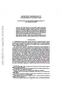
IV. N UMERICAL R ESULTS In this Section we show the theoretical curves of [P (c → 1 e)] min(n,l)m (that we will refer to as normalized probability of error) versus γ (dB) and we compare them with the numerical curves obtained using Eq. (10), (19) and (22) the eigenvalues of A = BB H where B is a computer generated complex Gaussian random matrix of finite size. Because the performances are normalized, losses in the normalized performance can occur even when the total number of antennas in the corresponding simulation is greater. The numerical performance are averaged over 100 Monte Carlo trials and in all simulation (m = 2). The slow Rayleigh fading case with ρ = 1 (i.e. n = l) is considered in Fig.1 where we compare the theoretical curve obtained by Eq. (11) (solid line) and the numerical results (dashed lines), for codes that are 2×2, 10×10 and 100×100. In Fig. 2 we show the theoretical and numerical curves for the slow Rician fading case with the same parameters as in Fig.1 and with Rician parameter ζ = 10. These figures show that, even for small sizes, our theoretical analysis provides an accurate estimate of the average performances. Fig. 3 shows the theoretical curves for slow Rayleigh fading for ρ = n/l = 1, 1.1, 2, 10, 100. We can observe how the gain obtained by increasing the number of antennas with respect to the code duration in the normalized 1 [P (c → e)] min(n,l)m vs. γ tend to saturate for ρ À 1. From our tests we observed that same effect is observed when n is fixed and the code length is increased.
Finally, in Fig. 4 we considered the case of fast Rayleigh fading and compared the theoretical curve corresponding to Eq. (23) with the numerical ones for n = l = 20. Note that the fast fading case is much more favorable than the slow fading case, which suggests that interleaved space time codes may gain significantly in terms of symbol error rate.
In this paper, building on the analysis developed in [1] and using the paradigm of Random Codes, we provided closed form expressions for the asymptotic frame error probability of space time coding. Our analysis is an useful tool to quantify the performance of the average space-time coding technique and can be used as a benchmark for testing the performance, without having to resort to an available code design.
theory numerical average −2
10
n=l=2
−3
10
[ P( c → e) ]1/(n m)
V. C ONCLUSIONS
Slow Rician fading, ρ=1
−1
10
n=l=10,100 −4
10
−5
10
−6
10
−7
10
5
10
15
20
γ (dB)
1 e)] min(n,l)m
25
30
Fig. 2. [P (c → vs. γ = Es /4N0 (dB); slow Rician fading, ρ = 1; theory (solid); numerical average for n = l = 2, 10, 100 (dashed).
R EFERENCES
ρ=1 ρ=1.1 ρ=2 −1
10
ρ=10 ρ=100
−2
Slow Rayleigh fading, ρ=1
0
Slow Rayleigh fading
0
10
[ P( c → e) ]1/(min(n,l) m)
[1] Vahid Tarokh, Nambi Seshardi, and A. R. Calderbank, “Space-Time Codes for High Data Rate Wireless Communication: Performance Criterion and Code Construction”, IEEE Trans. Inform. Theory, Vol. 44, NO. 2, pp. 744–765, March 1998. [2] Haagerup and S. Thorbjornsen, Random matrices with complex Gaussian entries, preprint (49 pp.), Odense 1998. Available at http://www.imada.ou.dk/ haagerup/2000-.html. [3] Predrag B. Rapajic and Popescu, “Information Capacity of a Random Signature Multiple-Input Multiple-Output Channel”, IEEE Trans. Comm., Vol. 48, NO. 8, pp. 1245–1248, August 2000. [4] G.J. Foschini, “Layered space-time architecture for wireless communication in a fading environment when using multielement antennas”, Bell Labs. Tech. Journ., Vol. 1, No. 2, pp. 41–59, 1996. ¨ Sako˘glu and A.Scaglione, “Asymptotic Capacity of Space-Time Coding for [5] U. Arbitrary Fading Channels: A Closed Form Solution Using Girko’s Law”,Proc. of IEEE ICASSP, Salt Lake City, May 2001. [6] A. J. Grant and P. D. Alexander, ”Random sequence multisets for syn-chronous for code-division multiple-access channels”, IEEE Trans. Inform. Theory, Vol. 44, pp. 2832-2836, Nov. 1998. [7] V. L. Girko - Theory of Random Determinants. KLUWER Publishers (Netherlands) 1990.
10
10
theory numerical average
9
10
11
12
13
Fig. 3. Effect of increasing ρ: [P (c → Rayleigh fading, ρ = 1, 1.1, 2, 10, 100.
γ (dB)
14
15
1 e)] min(n,l)m
16
17
18
vs. γ = Es /4N0 ; slow
−1
[ P( c → e) ]1/(n m)
10
Fast Rayleigh fading, ρ=1, n=l=20
0
10
theory numerical value
−2
10
−1
−3
10
5
10
1 e)] min(n,l)m
15
γ (dB)
20
25
30
[ P( c → e) ]1/(n m)
10
−2
10
Fig. 1. [P (c → vs. γ = Es /4N0 (dB); slow Rayleigh fading, ρ = 1; theory (solid); numerical average for n = l = 2, 10, 100 (dashed).
−3
10
5
10
1 e)] min(n,l)m
15
γ (dB)
20
25
30
Fig. 4. [P (c → vs. γ = Es /4N0 (dB); fast Rayleigh fading, ρ = 1; theory (solid); numerical average for n = l = 20 (dashed).