Asymptotic Robust Hypothesis Testing Based on ... - Semantic Scholar

Asymptotic Robust Hypothesis Testing Based on Moment Classes Sean Meyn and Venugopal V. Veeravalli ECE Department & Coordinated Science Lab University of Illinois at Urbana-Champaign Urbana, IL 61801, USA Email: meyn,[email protected]

Abstract— A robust hypothesis testing framework is introduced in which candidate hypotheses are characterized by moment classes. It is shown that there exists a test sequence that is asymptotically optimal in the min-max sense, and that it is expressed as a comparison of a log-linear combination of the constraint functions to a pre-determined threshold. Algorithms are described to compute the optimal test and applications of the robust hypothesis testing framework are discussed.

I. I NTRODUCTION We consider the binary hypothesis testing problem based on a finite number of observations from a sequence of observations X = {Xt : t = 1, . . .}, taking values in a finite set A. The goal is to classify a given set of observations into one of the two hypotheses, H0 or H1 . In much of this paper, it is assumed that, conditioned on the hypotheses H0 or H1 , these observations are independent and identically distributed (i.i.d.), with marginal distribution πj under hypothesis Hj for j = 0, 1. Standard approaches to deciding whether the observations come from H0 or H1 include the Bayesian, Neyman-Pearson, and min-max criteria (see, e.g., [1]). It is well-known that when the distributions π0 and π1 are specified, the optimal test under any one of these three criteria can be expressed as a Likelihood Ratio Test (LRT) [1]. In most applications, however, π0 and π1 are not completely specified a priori. Typically these distributions must be estimated through on-line or off-line measurements. The statistical modeling problem may then be solved by choosing an appropriate statistical model that is consistent with the measurements. Given that in reality the measurement data is always finite, there is a multitude of statistical models that are consistent with the data. In some exceptional cases, which arise mainly in the context of digital communications, the distributions under both hypotheses can be estimated very accurately. For example, in the communication of binary information over the telephone line channel, the observations (under each hypothesis) are the sum of a deterministic transmitted signal (that depends on the hypothesis) and a random noise term (that is independent of the hypothesis). The statistics of the noise term are relatively time-invariant and easy to estimate accurately prior to communication. In particular, zero-mean Gaussian models for the noise are known to be accurate, and the only

parameter that requires estimation is the noise variance. Hence the distributions π0 and π1 are essentially known. In other cases that arise in the context of surveillance, one of the hypotheses, typically denoted by H0 , corresponds to the case “null” where the intruder is absent, and the alternative H1 corresponds to the presence of an intruder. Such problems have recently generated much interest in the context of sensor networks (see, e.g., [2] and references therein). The default state of the system is H0 , and often there is ample opportunity to learn the observation statistics under this hypothesis. In this case, π0 can be assumed to be known. On the other hand, the parameters associated with the intruder are typically unknown a priori, and hence π1 may only be partially known. In general, both π0 and π1 may only be known partially. An example of such a scenario is digital communications over wireless channels subject to severe time varying interference with a few dominant interferers as in a cellular wireless communication systems. Here the additive noise term may not be well modeled as Gaussian or even statistically timeinvariant. Training to learn the statistics can only result in partial knowledge of π0 and π1 . Additive Gaussian models are typically used to model the interference only because they result in simple detector structures. A reasonable way to capture partial knowledge of π0 and π1 is through sets of distributions referred to as uncertainty classes. A standard approach to designing decision rules in this setting is the min-max approach, where the goal is to minimize the worst-case performance over the uncertainty classes. The decision rules thus obtained are said to be robust to the uncertainties in the probability distributions. Min-max robust detection has been the subject of numerous papers since the seminal work of Huber and Strassen [3], [4]. The solution to the robust detection problem, if one exists, is a LRT between a pair of least favorable distributions (LFDs) within the classes. Huber and Strassen showed that LFDs exist for several uncertainty models, such as ǫ-contaminated neighborhoods, total variation neighborhoods, band-classes, and p-point classes, or more generally when the neighborhood classes can be described in terms of alternating capacities of order 2 [4]. The proofs of existence of LFDs and the corresponding robust tests rely on the property that the uncertainty classes satisfy the joint stochastic boundedness assumption (as defined in [5]). Unfortunately the uncertainty models for which LFDs

are known to exist have limited application in practice, and the specific uncertainty model of interest in this paper (that we describe below) does not appear to be amenable to the Huber-Strassen approach. This paper concerns uncertainty classes obtained by specifying bounds on a finite number of moments of the distributions under the respective hypotheses. Specifically, we define the moment classes P0 and P1 as, n o Pj = π ∈ M : hπ, fij i ≤ cij , i = 1, ..., n , j = 0, 1, (1) where {fij } are real-valued functions1 on A, {cij } are constants, and M denotes the set of all distributions on A. We use the notation hπ, f i for the expected value of the function f with respect to the distribution π. Clearly, lower bound constraints on the moments hπ, fij i can be accomodated in this setting by additional constraints on −fij . It is assumed that the sets P0 , P1 are disjoint. Our motivation for considering moment classes comes firstly from the simple observation that the most common approach to partial statistical modeling is through moments, typically mean and correlation. Probabilistic inference using moment information has a long and rich history (see discussion in [6]). The primary motivation comes from the fact that it is possible to obtain worst-case bounds on the probability of a given set, over all probability distributions in a given moment class. As we mentioned previously, for uncertaintly classes defined by moment constraints, the min-max robust versions of the standard hypothesis testing problems do not fall under the Huber and Strassen framework. To facilitate analysis, we turn to the asymptotic setting that is described in more detail in the next section. Throughout this paper we restrict to our attention to the asymptotic version of the Neyman-Pearson (N-P) criterion for evaluating a given detector. The results of this paper can be extended to asymptotic robust versions of the Bayesian and min-max hypothesis testing problems. II. A SYMPTOTIC N-P H YPOTHESIS T ESTING The asymptotic robust N-P criterion [7] is described as follows. For a given N ≥ 1, suppose that a decision test φN is constructed based on the finite set of measurements {X1 , . . . , XN }. This may be expressed as the characteristic N function of a subset AN 1 ⊂ A . The test declares that hypothesis H1 is true if φN = 1, or equivalently, (X1 , X2 , . . . , XN ) ∈ AN 1 . In the asymptotic setting considered in this paper, we view N ≥ 1 as a parameter. The performance of a sequence ∆ of tests φ = {φN : N ≥ 1} is reflected in the error exponents for the type-II error probability and type-I error probability, defined respectively by, 1 log(Pπ1 (φN (X1 , . . . , XN ) = 0)), N →∞ N 1 ∆ log(Pπ0 (φN (X1 , . . . , XN ) = 1)), = − lim inf N →∞ N ∆

Iφπ1 = − lim inf Jφπ0 1 Note

that {fij } do not have to be polynomials.

where Pπj denotes the distribution on X when X is i.i.d. with marginal πj . Consider first the non-robust setting in which the distributions π0 , π1 are known exactly. The asymptotic N-P criterion for choosing an optimal test is to maximize the type-II exponent subject to a constraint on the type-I exponent. Thus, for a given constant η ≥ 0 as the constraint, we have sup Iφπ1

subject to

φ

Jφπ0 ≥ η

(2)

where the supremum is over all test sequences φ. The optimal value of the exponent Iφπ1 in the asymptotic N-P problem is expressed in Theorem 1 below, which is a combination of results established in [7] and [8]. Before we state the theorem we define some relevant quantities. For µ, π ∈ M, the relative entropy or Kullback-Leibler divergence between µ and π is defined as D µE ∆ D(µ k π) = µ, log (3) π For π ∈ M and for β ∈ ℜ+ , we define the divergence sets ∆

Qβ (π) = {µ ∈ M : D(µ k π) < β}, ∆

Q+ β (π) = {µ ∈ M : D(µ k π) ≤ β}.

(4)

Divergence sets are convex since D(· k π) is a convex function. Given the two distributions π0 , π1 we define the likelihood ratio by ∆ π0 (a) ℓ(a) = , a ∈ A. (5) π1 (a) Theorem 1: Suppose that the two distributions π0 , π1 are known exactly. Then the following statements hold, (i) The optimal value of Iφπ1 in (2) is given by the minimal divergence β∗ =

inf

µ∈Qη (π0 )

D(µ k π1 )

(6)

(ii) There exists a distribution µ∗ ∈ Q+ η (π0 ) that solves (6) and this solution satisfies D(µ∗ k π0 ) = η , and

D(µ∗ k π1 ) = β ∗

(iii) The following sequence of log-likelihood ratio tests (LRTs) is optimal for (2). N o n 1 X ∆ log ℓ(xt ) ≤ β ∗ − η . (7) φN = I x ∈ A N : N t=1

where I is the indicator function. Part (i) of Theorem 1 was proved by Hoeffding [7]. Results similar to (ii) and (iii) were established by Blahut[8]. Below we provide a sketch of the proof based on Sanov’s Theorem and the geometry of convex sets, which will be useful when we study the robust detection problem.

We briefly recall Sanov’s theorem here. Define the types for X = (X1 , X2 , . . .) through the sequence of empirical distributions (indexed by N ) a ∈ A.

µ∈E

(9)

The relative entropy is jointly convex on M × M, and hence computation of the minimum of D(µkπ) amounts to solving a convex program. The optimal value of the exponent Iφ in the asymptotic N-P problem is described in terms of relative entropy. It is shown in [9] that one may restrict to tests of the following form without loss of generality: for a closed set E ⊆ M, φN = I{γN ∈ E},

(10)

where {γN } denotes the sequence of types (8). Sanov’s Theorem (9) tells us that for any test of this form, Iφπ1

= inf c D(µkπ1 ), µ∈E

Jφπ0

= inf D(µkπ0 ). µ∈E

Jφπ0

The smallest set E that gives ≥ η is the divergence set (π ) (see (4)), and hence the optimum value of Iφπ1 in (2) Q+ 0 η is the value of the convex program, β ∗ = sup{β ≥ 0 : Qη (π0 ) ∩ Qβ (π1 ) = ∅} = inf D(µ k π1 ). µ∈Qη (π0 )

+ and the optimizing µ∗ ∈ Q+ η (π0 ) ∩ Qβ ∗ (π1 ) clearly satisfies the conditions given in part (ii) of Theorem 1. It is clear fromn (10) and (9) that any E ∈ M such that E ⊇ Qη (π0 ) and E c ⊇ Q∗β (π1 ) defines a sequence of optimal tests for (2) via φN = I{γN ∈ E}. In particular, setting E = Q+ η (π0 )} yeilds a universal test in that it does not require knowledge of π1 [9]. However, this universal test is considerably more difficult to implement than the LRT of (7). The key to showing that (7) is optimal is to establish that the following set

H = {µ ∈ M : hµ, log ℓi = hµ∗ , log ℓi} is a separating set (hyperplane) for the convex sets Q+ η (π0 ) and Q+ (π ). This result follows from the Kuhn-Tucker alignment ∗ 1 β conditions based on a dual functional. Note that we can write the constant hµ∗ , log ℓi as     µ∗ µ∗ − µ∗ , log hµ∗ , log ℓi = µ∗ , log π1 π0 = β∗ − η Thus an optimal sequence of decision rules results if we choose φN = I{hγN , log ℓi ≤ β ∗ − η} which is the test specified in (7). This geometry is illustrated in Figure 1.

hµ, log(ℓ)i = hµ∗ , log(ℓ)i

π0

(8)

Suppose that X is i.i.d. with marginal distribution π. Sanov’s Theorem states that for any closed convex set of distributions E ⊆ M, lim −N −1 log P{γN ∈ E} = inf D(µkπ)

π1 µ∗

Qη (π 0 )

N 1 X γN (a) = I{Xk = a}, N t=1

N →∞

Qβ ∗ (π 1 )

Fig. 1. The likelihood ratio test interpreted via a separating hyperplane between the convex sets Qη (π0 ) and Qβ ∗ (π1 ).

III. ROBUST A SYMPTOTIC N-P H YPOTHESIS T ESTING We now get to the main result of this paper, which is an extension of Theorem 1 to the robust framework. When π0 and π1 are known to belong to the uncertainty classes P0 and P1 respectively, we impose a uniform constraint on the type-I exponent for all π0 ∈ P0 , and subject to this we seek a test sequence that maximizes the worst type-II exponent across π1 ∈ P1 . Thus, in the robust version, the asymptotic N-P criterion (2) is replaced by the following constrained optimization: sup inf Iφπ1

inf Jφπ0 ≥ η.

subject to

φ π1 ∈P1

π0 ∈P0

(11)

Theorem 2 below describes optimal solutions to this optimization problem. For any moment class P defined as in (1), consider the divergence sets [ [ Q+ (P) = Qβ (π) , and Q+ Qβ (P) = β (π). (12) β π∈P

π∈P

It is easy to show that these divergence sets are also convex based on the joint convexity of the relative entropy and the convexity of P. The following assumption is imposed to ensure that the solution to the robust hypothesis testing problem is non-trivial: (A1) Q+ η (P0 ) ∩ P1 = ∅. This simply means that D(π1 k π0 ) > η for each π0 ∈ P0 , and π1 ∈ P1 . Theorem 2: The following hold for the asymptotic robust N-P hypothesis testing problem (11) under Assumption (A1): (i) The optimal value of Iφπ1 in (11) is given by ∆

β ∗ = sup{β ≥ 0 : Qη (P0 ) ∩ Qβ (P1 ) = ∅} inf D(µ k π1 ). = inf

(13)

π1 ∈P1 µ∈Qη (P0 )

(ii) There exist π0∗ ∈ P0 , π1∗ ∈ P1 , and µ∗ ∈ M that solve (13) and this solution satisfies D(µ∗ kπ0∗ ) = η,

D(µ∗ kπ1∗ ) = β ∗ .

The distributions π0∗ , π1∗ and µ∗ are are related through µ∗ (a) = ℓ0 (a) π0∗ (a) = ℓ1 (a) π1∗ (a), a ∈ A where ℓ0 (a) =

n X i=1

λi fi0 (a) , and

ℓ1 (a) =

n X

γi fi1 (a)

i=1

for appropriately chosen {λi , γi , i = 1, . . . , n}

(iii) The following three sequences of tests are all optimal for (11). (0) ∆

φN = I{x ∈ AN : hγN , log ℓ0 i > η} (1) ∆

φN = I{x ∈ AN : hγN , log ℓ1 i ≤ β ∗ }

(14)

∆

φN = I{x ∈ AN : hγN , log ℓi ≤ β ∗ − η} ∆

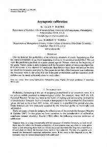
where ℓ(a) = ℓ1 (a)/ℓ0 (a) for a ∈ A. Analogous to the proof of Theorem 1, restricting to tests of the form φN = I{γN ∈ E}, the smallest set E that gives inf π0 ∈P0 Jφπ0 ≥ η is the divergence set Q+ η (P0 ). Thus the optimum value of Iφπ1 in (11) is as given in part (i) of Theorem 2. Also note that any E ∈ M such that E ⊇ Qη (P0 ) and E c ⊇ Q∗β (P1 ) defines a sequence of optimal tests for (11) via φN = I{γN ∈ E}. In particular, setting E = Q+ η (P0 )} yeilds a universal test. However, simpler optimal tests exist as seen in part (iii) of Theorem 2. + Since Q+ η (P0 ) and Qβ ∗ (P1 ) are compact sets it follows from their construction that there exists µ∗ ∈ Q+ η (P0 ) ∩ Q+ β ∗ (P1 ). Moreover, by convexity there exists some function h : A → ℜ defining a separating hyperplane between the sets + Q+ η (P0 ) and Qβ ∗ (P1 ), satisfying Qη (P0 ) ⊂ {µ ∈ M : hµ, hi < τ }, Qβ ∗ (P1 ) ⊂ {µ ∈ M : hµ, hi > τ }. The remainder of the proof consists of the identification of h and τ using the Kuhn-Tucker alignment conditions based on consideration of a dual functional as in the proof of Theorem 1. However, unlike in the case of Theorem 1, there is some flexibility in the choice of h as we see in part (iii) of Theorem 2. This geometry of the test corresponding to ℓ0 is illustrated in Figure 2 below. We also note that likelihood ratio between π0∗ and π1∗ can be written as: π0∗ (a) ℓ1 (a) = = ℓ(a) ∗ π1 (a) ℓ0 (a) Thus it is tempting to consider the third optimal test sequence in part (iii) to be a likelihood ratio test based on π0∗ and π1∗ . However, the support of π0∗ and π1∗ may be a small subset of A in applications, whereas ℓ(a) is defined for all a ∈ A. Qβ ∗ (P1 )

π 1∗

P1

µ∗

Qη (P0 )

π

0∗

hµ, log(ℓ0 )i = hµ∗ , log(ℓ0 )i P0

Fig. 2. The robust hypothesis testing problem. The uncertainty classes Pi , i = 0, 1 are determined by a finite number of linear constraints, and the thickened regions Qη (P0 ), Qβ ∗ (P1 ) are each convex. The linear threshold test corresponding to ℓ0 is interpreted as a separating hyperplane between these two convex sets.

IV. N UMERICAL C OMPUTATION The optimal π0∗ , π1∗ , µ∗ , and β ∗ of Theorem 2 can be obtained using standard techniques from nonlinear programming. A recursive approach based on the cutting-plane method of Kelley [10] yields an efficient algorithm for numerical computation. V. C ONCLUSION We have characterized the solution to the asymptotic robust hypothesis problem where the distributions under the two hypotheses belong to moment classes. We showed that optimal test sequences can be expressed as a comparison of a linear combination of the constraint functions to a threshold. Potential directions for future work are drawn from both theoretical as well as practical viewpoints. Specifically, we believe the following directions would be of interest: 1) It is likely that many of our conclusions can be extended beyond the i.i.d. case to include classes of Markov processes, and beyond the finite-alphabet case. 2) We have not dealt with the problem of how to select the moment functions {fij } for an arbitrary application. It may be possible to formulate rules for selecting these functions based on additional information about the candidate hypotheses. For instance, when the distribution π0 is known, the functions {fi1 } could be tailored so that discriminating between π0 and π1 ∈ P1 is made easier. 3) Extension to M -ary hypothesis testing (M > 2) is of interest, particularly in the context of channel coding. ACKNOWLEDGMENT The authors thank Charuhas Pandit for his contributions to this research. This paper is based upon work supported by the National Science Foundation under Award Nos. ECS-0217836, ITR-0085929, and the CCF-0049089. R EFERENCES [1] H. V. Poor, An introduction to signal detection and estimation. New York: Springer-Verlag, 2nd ed., 1994. [2] J.-F. Chamberland and V. V. Veeravalli, “Decentralized detection in sensor networks,” IEEE Transactions on Signal Processing, vol. 51, pp. 407–416, 2003. [3] P. J. Huber, “A robust version of the probability ratio test,” Ann. Math. Stat., vol. 36, pp. 1753–1758, 1965. [4] P. J. Huber and V. Strassen, “Minimax tests and the Neyman-Pearson lemma for capacities,” Annals of Statistics, vol. 1, pp. 251–263, 1973. [5] V. V. Veeravalli, T. Basar, and H. V. Poor, “Minimax robust decentralized detection,” IEEE Transactions on Information Theory, vol. 40, no. 1, pp. 35–40, 1994. [6] C. Pandit, Robust Statistical Modeling Based on Moment Classes with Applications to Admission Control, Large Deviations, and Hypothesis Testing. PhD thesis, University of Illinois at Urbana-Champaign, Urbana, IL, USA, 2004. [7] W. Hoeffding, “Asymptotically optimal tests for multinomial distributions,” Ann. Math. Statist., vol. 36, pp. 369–408, 1965. [8] R. E. Blahut, “Hypothesis testing and information theory,” IEEE Transactions on Information Theory, vol. IT-20, no. 4, pp. 405–417, 1974. [9] O. Zeitouni and M. Gutman, “On universal hypotheses testing via large deviations,” IEEE Trans. Inform. Theory, vol. 37, no. 2, pp. 285–290, 1991. [10] J. Kelley, Jr., “The cutting-plane method for solving convex programs,” J. Society Industrial Appl. Mathematics, vol. 8, no. 4, pp. 703–712, 1960.