Asymptotically optimal parallel resource assignment with interference

Asymptotically optimal parallel resource assignment with interference I.M. Verloop1,2 , R. N´ un ˜ ez-Queija2,3 1

BCAM – Basque Center for Applied Mathematics, Derio, Spain 2 CWI, Amsterdam, The Netherlands 3 University of Amsterdam, The Netherlands

Abstract Motivated by scheduling in cellular wireless networks and resource allocation in computer systems, we study a service facility with two classes of users having heterogeneous service requirement distributions. The aggregate service capacity is assumed to be largest when both classes are served in parallel, but giving preferential treatment to one of the classes may be advantageous when aiming at minimization of the number of users, or when classes have different economic values, for example. We set out to determine the allocation policies that minimize the total number of users in the system. For some particular cases we can determine the optimal policy exactly, but in general this is not analytically feasible. We then study the optimal policies in the fluid regime, which prove to be close to optimal in the original stochastic model. These policies can be characterized by either linear or exponential switching curves. We numerically compare our results with existing approximations based on optimization in the heavy-traffic regime. By simulations we show that, in general, our simple computable switching-curve strategies based on the fluid analysis perform well.

1

Introduction

In many practical applications where resources must be allocated to several contending users or tasks, the service capacity itself may be affected by the scheduling policy deployed. Our work is motivated by two specific application areas. In third generation wireless networks, neighboring base stations may interfere with each other when transmitting simultaneously. When one base station is not active, other base stations can work at higher rates, see for example [7, 8]. For data applications, base stations may coordinate transmissions (i.e., transmit simultaneously or alternatingly) so as to improve the use of the shared spectrum. A second motivating application is the scheduling of resources in computer systems (or Web servers) where jobs must be routed to one of several servers, see for example [27, 28]. There, the capacity depends on the allocation when servers are specialized for certain tasks. Scheduling of resources with policy-dependent capacities has attracted much attention in recent years. Most of the results concern stochastic stability properties of such systems. Due to the dependence of capacity on the service policy, even this most basic performance measure is a non-trivial task to determine. In [11] bounds for stability in a general class of systems with policy-dependent capacity have been determined. In the specific context of wireless networking, stability of utility-based allocation strategies was shown to be intimately related with the shape of the feasible capacity region [10], i.e., the set of simultaneously achievable transmission rates for all users. With a convex capacity region, the system is stabilized by any such allocation

1

strategy, but this is not the case for non-convex capacity regions. These results were later generalized to non-convex and time-varying capacity regions in [22], showing the precise conditions for stability of utility-based strategies under quite general assumptions on the time-variations. Stability conditions for non utility-based strategies, for example threshold-based policies, were investigated in [28, 34]. As may be expected from the complexity of determining stability, results on the flow level performance in terms of system delay or system occupancy are scarce. In this paper, we focus on a particular model with simultaneous resource sharing that turns out to be equivalent to a parallel-server model where user classes can be served in parallel, all by a dedicated server, or where several servers can be simultaneously allocated to one class only. This type of models is known to be notoriously hard to analyze, as is illustrated by special cases (including the so-called coupled-processors model) requiring the solution of a Riemann-Hilbert boundary value problem [13, 16]. Most results on flow-level performance in parallel-server models concentrate on a specific class of scheduling policies. For example, besides determining the stability conditions, the authors in [28] investigate the performance of threshold-based policies. One main observation there is that finding reasonable values for the thresholds is not trivial since performance as well as stability can be quite sensitive to the threshold values. Approximations for mean response times are given in [27]. A general class of threshold-based priority policies for multi-class parallel-server networks is also proposed in [33]. For these strategies, the authors derive approximate formulas for the queue lengths and illustrate how these can be used to obtain reasonable threshold values. In [7, 8] a parallel two-server model is analyzed under the policy that always serves both classes in parallel whenever both are present, and a diffusion approximation for the queue lengths is found for a specific heavy-traffic setting. Our goals here are to study the structural properties of optimal scheduling policies in a parallelserver model, and to determine computable approximations that are close to optimality. Our objective is to minimize (in some appropriate sense) the total number of users. A crucial observation when addressing optimality is that, in general, users will have class-specific sizes, so that few users of one class can typically add up to the same amount of work as many of another class. On one hand, it seems reasonable to maximize the departure rate of users, by serving the “small” users first. In the short run, this will keep the number of users in the system at a low level, thus shortening overall delays. On the other hand, it is also desirable to deploy the highest possible total service capacity. That will minimize the volume of back-logged work and drain the system at maximum rate, thus ensuring maximum stability. In general, finding the optimal trade-off between these two intrinsically different objectives is a challenging task. Determining the exact optimal policy in a parallel-server model has so far proved analytically infeasible. Most research on this area has focused on heavily-loaded systems under a (complete) resource pooling condition for which asymptotically optimal policies in heavy traffic are determined [1, 5, 6, 19, 20, 24, 32]. In [1, 19, 20] several discrete-review policies are proposed (the system is reviewed at discrete points in time, and decisions are based on the queue lengths at the revision moment) and are proved to be asymptotically optimal in heavy traffic. In [24, 32] a generalized cµ-rule is proposed (including the Max-Weight policy as a special case) that myopically maximizes the rate of decrease of certain instantaneous holding cost. This policy is robust in the sense that it only depends on the departure rates and the cost function, and it is proved that this policy minimizes the cumulative cost over any finite interval in a heavily-loaded system. In [5, 6], the authors prove that threshold-based strategies minimize the scaled total number of users in a heavy-traffic setting. The order of magnitude of the optimal thresholds as functions of the traffic load can be determined, but this does not give a recipe to choose good threshold values in moderately-loaded regimes. In [33], the authors propose values for the threshold, which can be found by solving a minimization problem. 2

In this paper, we consider a parallel two-server model with two traffic classes that can be served either in parallel or alternatingly. The highest service capacity is achieved when serving both classes in parallel, but with asymmetric service requirements, the user departure rate may be larger when serving one class only. For some special cases the optimal policy can be determined exactly, but this is not possible in general. In a similar setting, [4] states that switchingcurve policies are optimal (a proof will be included in a forthcoming paper by the authors of [4]). Numerical experiments included for illustration in the present paper indeed support this optimality. In order to find computable approximations for the optimal policies we study the model in a fluid-limit regime for which we show that the optimal policy is characterized by a linear switching curve. The optimal switching curves in the fluid regime can be used to determine asymptotically fluid optimal policies for the stochastic model. These policies are characterized by either linear or exponential switching curves. Our analysis is inspired by that in [17, 18] where a multi-class tandem-network is studied. By simulations we compare these asymptotically fluid optimal switching-curve policies with threshold-based policies [5, 6] and Max-Weight policies [24, 32] which are optimal in heavy traffic. We show that the fluid-based and threshold-based policies give good performance in general, while significant improvements over Max-Weight policies can be achieved. It is worth noting that the optimal policies studied in this paper rely on centralized control. In practice, centralized control may require a prohibitive amount of overhead. However, knowledge of the (centralized) optimum is extremely valuable to (numerically) estimate the scope for improvement of decentralized control policies. For example, in the application area of bandwidthsharing networks, it was found numerically that certain distributed schemes may actually be close to the theoretical (centralized) optimum [35, 36]. The paper is organized as follows. In Section 2 we describe the model and state some preliminary results. Section 3 contains our optimality results for the stochastic model. The fluid analysis and the asymptotically fluid optimal policies are presented in Section 4. For comparison we briefly discuss optimal policies in heavy traffic using the results of [5, 6] and [24, 32] in Section 5. Numerical experiments and concluding remarks can be found in Sections 6 and 7.

2

Model description and preliminaries

We consider the following model. There are two classes of users. Class-i users, i = 1, 2, arrive according to independent Poisson processes with rate λi and have exponentially distributed service requirements with mean 1/µi , i = 1, 2. Without loss of generality, we assume throughout the paper that µ1 ≥ µ2 , that is the service requirements of class-1 users are relatively small. Define the traffic load of class i as ρi := µλii . At any time, either one class can be served individually with capacity 1, or both classes 1 and 2 can be served in parallel with capacities c1 and c2 respectively, ci ≤ 1, or the system is idling (not serving any class), or any convex combination of these four. For a given policy π, denote by sπi (t) the service capacity devoted to class i at time t. We assume that sπi (t) = 0 when Ni (t) = 0. In addition, we assume the process sπi (t) to be right continuous with left limits. The vector sπ (t) = (sπ1 (t), sπ2 (t)) lies in the capacity region S, which is defined as the convex hull of the set {(0, 0), (1, 0), (0, 1), (c1 , c2 )} (see Figure 1 in the case c1 +c2 > 1). Note that the total (service) capacity sπ1 (t) + sπ2 (t), that is, the speed at which the total amount of backlogged work in the system decreases, is not constant in time. Depending on the decision taken at time t, it may vary between 0 and max(1, c1 + c2 ). The rate at which users leave the system is µ1 sπ1 (t) + µ2 sπ2 (t), which we refer R ttoπ as the (user) departure rate. π Let Si (t) := 0 si (u)du denote the cumulative amount of capacity devoted to class i in the time interval (0, t) under policy π. Let Ai (u, t) be the amount of class-i work that arrived during the 3

s2 1 (c1 , c2 )

1

s1

Figure 1: Capacity region S when c1 + c2 > 1.

time interval (u, t]. Then, the workload in class i at time t can be written as Wiπ (t) := Wi (0) + Ai (0, t) − Siπ (t).

(1)

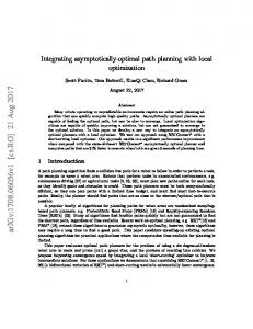
Denote by Niπ (t) the number of class-i users at time t, and let N π (t) = (N1π (t), N2π (t)). We further define Niπ and N π as random variables with the corresponding equilibrium distributions (when they exist). Remark 2.1 With resource allocation in computer systems in mind, it is more natural to view the model as an equivalent parallel-server model with two servers and two classes, as depicted in Figure 2. Server 1 can either serve class 1 with capacity c1 , or class 2 with capacity 1 − c2 . Similarly, server 2 can either serve class 2 with capacity c2 , or class 1 with capacity 1 − c1 . Hence, when the two servers are dedicated to their own classes, classes 1 and 2 are served in parallel with capacities c1 and c2 , respectively. When instead both servers are allocated to the same class, this class is served with capacity 1. (In our setting, both servers can work together on one single user, thus achieving a service capacity of 1 even when there is only one user in the system.) Note that, although uncommon in this setting, it is no restriction to require that the service capacity obtained by combining the two servers equals 1 irrespective of the queue being served. In fact, this can be achieved for any parallel-server model by normalizing the service requirements.1 For any point in time, one needs to decide how the service capacity should be divided between the two classes. The objective of the paper is to identify scheduling policies that in some appropriate sense minimize the total number of users in the system. We focus on policies that only use knowledge of the past evolution of the number of users. Since the service requirements and inter-arrival times are exponentially distributed, the Markov property implies that we only need to consider policies that base decisions on the number of users present in the various classes. In particular, we exclude anticipating policies, i.e., policies that have knowledge available of the remaining service requirements. The set of these Markovian non-anticipating policiesR is denoted m 1 E( 0 (N1π (t)+ by Π. We call a policy π ˜ ∈ Π average optimal when π ˜ = argminπ∈Π lim supm→∞ m ˜ ∈ Π is stochastically optimal when N1π˜ (t) + N2π˜ (t) ≤st N1π (t) + N2π (t), for N2π (t))dt). A policy π 1

One may think of µi to be the user departure rate of class i when served exclusively (with normalized service capacity 1). Then c1 and c2 may be adjusted so that µi ci equals the user departure rate of class i when the two classes are served simultaneously. To be specific, consider a parallel two-server model where C˜i is the service capacity in queue i when allocated both servers, c˜1 and c˜2 are the service capacities in both queues under parallel service, and 1/˜ µ1 and 1/˜ µ2 are the mean service requirements. The queue length process is then equivalent with our normalized system when setting µi = µ ˜i C˜i and ci = c˜i /C˜i .

4

c1

class 1

server 1 1 − c2 1 − c1

class 2

server 2 c2

Figure 2: Parallel two-server model.

all t ≥ 0, π ∈ Π, whenever N π˜ (0) = N π (0). By definition, for two positive random variables X and Y , we use X ≤st Y to denote that P(X > s) ≤ P(Y > s) for all s ≥ 0. A stochastically optimal policy, if it exists, is automatically average optimal as well. In the paper we assume c1 + c2 > 1. However, before proceeding let us briefly consider the situation c1 + c2 ≤ 1. In the latter case, the policy that gives preemptive priority to class 1 (the class with the highest departure rate) is stochastically optimal. (In fact, this result holds for any shape of the capacity region where the points (1, 0) and (0, 1) are not dominated by any other element in the capacity region.) Intuitively, this can be understood by noting that if c1 + c2 ≤ 1, then serving class 1 exclusively will maximize the rate at which the total workload in the system decreases. At the same time, since µ1 ≥ c1 µ1 + c2 µ2 , serving class 1 myopically maximizes the departure rate. A formal proof can be obtained along the lines of Proposition 3.3 below using dynamic programming. Average optimality is actually rather easy to deduce and we give its proof here: Denote by π (1) the policy that gives preemptive priority to class 1. Then for any policy π ∈ Π, if at time t = 0 the workloads satisfy (1)

(1) W1π (t)

+

W1π (t) ≤ W1π (t), (1) W2π (t)

≤

W1π (t) +

(2) W2π (t),

(3)

then the same is true for all t ≥ 0. These inequalities hold sample-path wise (for all t), and they imply stochastic inequalities for the workload processes. Multiplying (2) by µ1 − µ2 ≥ 0 (1) (1) and (3) by µ2 and adding the two inequalities gives that µ1 W1π (t) + µ2 W2π (t) ≤ µ1 W1π (t) + µ2 W2π (t). Since we have exponentially distributed service requirements and we consider only (1) (1) non-anticipating policies, we obtain E(Wiπ (t)) = µ1i E(Niπ (t)), so that E(N1π (t))+E(N2π (t)) ≤ E(N1π (t)) + E(N2π (t)), for all t ≥ 0 and for all policies π ∈ Π. In particular, policy π (1) is average optimal. As mentioned before, in the remainder of the paper we will focus on the unsolved case c1 +c2 > 1. In this case, the total service capacity is largest when both classes are served in parallel. For application in wireless networks, this represents the joint capacity when both base stations transmit in parallel, and in computer scheduling it corresponds to dedicated specialized servers.

2.1

Stability

For a given policy π, the system is called stable when the process N π (t) is positive recurrent. Since c1 + c2 > 1, the policy that serves classes 1 and 2 in parallel, whenever possible, minimizes the total workload in the system at every moment in time. Hence, this policy will keep the system stable whenever possible. Under this policy, the model becomes a coupled-processors

5

model for which the stability conditions are min( if

ρ1 ρ2 , ) < 1 and c1 c2

ρi ρi < 1 then ρj + (1 − cj ) < 1, i 6= j, ci ci

(4) (5)

as proved in [13, 16]. Conditions (4) and (5) are therefore necessary conditions for the system to be stable. However, they do not guarantee stability for an arbitrary policy, and the exact (sufficient and necessary) stability conditions depend strongly on the scheduling policy used. Note that the load vectors (ρ1 , ρ2 ) that satisfy the necessary stability conditions (4) and (5), are exactly those vectors that lie in the interior of the capacity region S depicted in Figure 1.

3

Optimality results

For a standard multi-class single-server queue it is well known that if class-i users have exponentially distributed service requirements with mean 1/µi , for all classes i, then the policy that gives preemptive priority to the class with the highest departure rate µi (the so-called µ-rule), is stochastically optimal [30]. The rationale behind this rule is that it maximizes the departure rate at all times. One might expect that such a rule is optimal in our model as well. The µ-rule would amount to choosing the allocation s(t) that maximizes the user departure rate, µ1 s1 (t) + µ2 s2 (t), at any time t. Unfortunately, the total service capacity, s1 (t) + s2 (t), depends on the chosen allocation as well. For example, serving class i only decreases the total amount of work at rate 1, while serving both classes in parallel gives a decrease of the workload at rate c1 + c2 > 1. Therefore, the objective to maximize the user departure rate may be conflicting with that of maximizing the total service capacity used. The latter will minimize the total time needed to empty the system, which is advantageous in the long run, while the former is better in the short run. Recall that we chose µ1 ≥ µ2 . If, in addition, µ1 ≤ µ1 c1 + µ2 c2 , then there is no trade-off and it is intuitively clear that the policy that always serves classes 1 and 2 in parallel (whenever both are backlogged) is optimal, since this maximizes both the workload depletion rate and the departure rate. In Section 3.1 we show that the above described policy is in fact stochastically optimal. When µ1 ≥ µ1 c1 + µ2 c2 , the highest departure rate is obtained when serving class 1 individually. It may therefore be better to sometimes serve class 1 individually, even if that does not maximize the rate at which the total work in the system decreases. Hence as the number of users varies, the system should dynamically switch between different allocations. This setting is included in Section 3.2.

3.1

Stochastic optimality when µ1 ≤ µ1 c1 + µ2 c2

In this section we show that when (µ2 ≤) µ1 ≤ µ1 c1 + µ2 c2 , the policy that serves both classes in parallel (whenever possible) is stochastically optimal. Although it seems natural to prove this using stochastic coupling techniques, we have not been able to find such a coupling. For that reason we resort to dynamic programming techniques. We choose a framework which is somewhat broader than strictly needed to prove the required stochastic optimality of the number of users (we only need a particular choice of the function C(·) below). Doing so, we emphasize the essential properties needed to prove stochastic optimality. We consider the uniformized Markov chain, which is equivalent to the original process, see [29, Section 11.5]. In the uniformized chain, the transition epochs (including ’dummy’ transitions that do not alter the system state) are generated by a Poisson process of constant rate ν = 6

λ1 + λ2 + µ1 (1 + c1 ) + µ2 (1 + c2 ). Since ν is finite, we may assume ν = 1 without loss of generality. We then focus on the discrete-time Markov chain embedded at transition epochs and, for transparency of notation, again denote the number of class-i users after k steps by Ni (k), i = 1, 2. Let x = (x1 , x2 ) ∈ Z2+ . We define the functions Vk (x), k = 0, 1, . . ., as follows: V0 (x) = C(x) Vk+1 (x) = λ1 Vk (x + e1 ) + λ2 Vk (x + e2 ) nX o X + min 1(xi >0) µi si Vk (x − ei ) + (1 − λ1 − λ2 − 1(xi >0) µi si )Vk (x) s∈S

i=1,2

i=1,2

= λ1 Vk (x + e1 ) + λ2 Vk (x + e2 ) + (µ1 (1 + c1 ) + µ2 (1 + c2 ))Vk (x) nX o + min 1(xi >0) µi si (Vk (x − ei ) − Vk (x)) , s∈S

(6)

i=1,2

for x1 , x2 ≥ 0, k = 0, 1, . . . , with C(·) : Z2+ → R a terminal cost function, S the capacity region, and ei the i-th unit vector. The term Vk+1 (x) represents the minimum achievable expected terminal cost, when the system starts in state x at k + 1 steps from the horizon. In addition, a minimizing action in (6) is an optimal action at k + 1 steps from the horizon. Setting the cost function in this framework equal to C(x) = 1(x1 +x2 >y) , we obtain that Vk+1 (x) represents the minimum achievable value for P(N1 (k + 1) + N2 (k + 1) > y|N (0) = x). If we then show that for all y ≥ 0 and all k ∈ {0, 1, . . .}, we can choose the same minimizing action in (6) (the optimal action may depend on the state x), then the corresponding policy is stochastically optimal at every instant in time. In the next two lemmas we establish convenient properties of Vk (·), under certain conditions on the function C(·). Lemma 3.1 If C(x) is non-decreasing in x1 and x2 , then Vk (x) is non-decreasing in x1 and x2 for all k. Proof: The statement follows directly from the definition of Vk (·).



The set S is convex, hence the minimizing action in (6) will be one of the extreme points of P S. From Lemma 3.1 it can be concluded that the minimizer will not be (0, 0) ∈ S, since i=1,2 1(xi >0) µi si (Vk (x − ei ) − Vk (x)) ≤ 0, for all s ∈ S. Hence, we can rewrite the function Vk+1 (·) as follows: Vk+1 (x) = λ1 Vk (x + e1 ) + λ2 Vk (x + e2 )  + min µ1 Vk ((x1 − 1)+ , x2 ) + (µ2 + µ1 c1 + µ2 c2 )Vk (x),

µ2 Vk (x1 , (x2 − 1)+ ) + (µ1 + µ1 c1 + µ2 c2 )Vk (x),

 µ1 c1 Vk ((x1 − 1)+ , x2 ) + µ2 c2 Vk (x1 , (x2 − 1)+ ) + (µ1 + µ2 )Vk (x) .

(7)

In the next lemma we will show that under certain conditions on C(x), the minimizing action in (7) will be to always serve classes 1 and 2 in parallel, whenever possible. The proof uses Lemma 3.1 and may be found in Appendix A. Lemma 3.2 If c1 + c2 ≥ 1 and Z(x) = C(x) is non-decreasing in x1 and x2 and satisfies (µ1 + µ2 )Z(x) + µ1 c1 Z(x − e1 ) + µ2 c2 Z(x − e2 ) ≤ min(µ1 Z(x − e1 ) + (µ2 + µ1 c1 + µ2 c2 )Z(x),

µ2 Z(x − e1 ) + (µ1 + µ1 c1 + µ2 c2 )Z(x)),

for x1 , x2 > 0, then Z(x) = Vk (x) satisfies (8) as well, for any k ≥ 0. 7

(8)

We can now find a stochastically optimal policy when (µ2 ≤)µ1 ≤ µ1 c1 + µ2 c2 . Proposition 3.3 Assume c1 + c2 ≥ 1. If (µ2 ≤)µ1 ≤ µ1 c1 + µ2 c2 , then it is stochastically optimal to serve both classes in parallel whenever possible. Proof: If (µ2 ≤)µ1 ≤ µ1 c1 + µ2 c2 , then the cost function C(x1 , x2 ) = 1(x1 +x2 >y) satisfies the conditions as given in Lemma 3.2, for all y ≥ 0. From Lemma 3.2 we obtain that serving both classes in parallel (whenever possible) is always the minimizing action in (7) and hence the corresponding stationary policy is stochastically optimal. 

3.2

General characterization of the average-optimal policy

Section 3.1 treats the case µ1 ≤ µ1 c1 + µ2 c2 , for which a stochastically optimal policies exist. Since this may in general not be the case, we now discuss the general structure of an averageoptimal policy. When µ1 > µ2 , maximizing the user departure rate would imply that an optimal policy will never serve class 2 individually when class 1 is also present. At the same time, serving class 2 individually does not give the highest possible total service capacity either, since c1 + c2 > 1. Therefore, it is natural that an optimal policy should never serve class 2 individually when there is also work of class 1 present. This fact is proved in Proposition 3.5. First we state a lemma that in fact holds for generally distributed inter-arrival times and service requirements, and in particular, holds irrespective of the values for µ1 and µ2 . The proof may be found in Appendix B. Lemma 3.4 (This lemma holds for generally distributed inter-arrival times and service requirements.) Assume c1 + c2 > 1. Let π ˜ be a policy that sometimes does serve class 2 individually while there are class-1 users present. Define policy π to be the policy that uses the same allocation as π ˜ when possible, except when policy π ˜ serves class 2 individually. In that case policy π serves classes 1 and 2 in parallel (if possible). Consider the same realizations of the arrival processes and service requirements. Then the following sample-path inequalities hold: S1π (t) ≥ S1π˜ (t)

(1 −

S1π (t) + S2π (t) ≥ S1π˜ (t) + S2π˜ (t)

c2 )S1π (t) + c1 S2π (t)

≥ (1 −

c2 )S1π˜ (t)

(9) (10) + c1 S2π˜ (t),

(11)

for all t ≥ 0. Proposition 3.5 Assume µ1 ≥ µ2 and c1 + c2 > 1. For any policy π ˜ that serves class 2 individually when there is work of class 1 present, there exists a modified policy π that never serves class 2 individually when class 1 is present and that does not do worse than π ˜ , i.e., E(N1π (t) + N2π (t)) ≤ E(N1π˜ (t) + N2π˜ (t)), for all t ≥ 0. Proof : Let π ˜ be a policy that sometimes does serve class 2 individually while there are class-1 users present. Define policy π as in Lemma 3.4 and hence the sample-path inequalities (9) and (10) hold. Multiplying (9) by µ1 − µ2 ≥ 0 and (10) by µ2 and adding the two inequalities gives that µ1 S1π (t) + µ2 S2π (t) ≥ µ1 S1π˜ (t) + µ2 S2π˜ (t) and hence by (1) we obtain µ1 W1π (t) + µ2 W2π (t) ≤ µ1 W1π˜ (t) + µ2 W2π˜ (t),

(12)

for all t ≥ 0. Since we assumed exponentially distributed service requirements and we consider only non-anticipating policies, we have E(Wiπ (t)) = µ1i E(Niπ (t)). By taking expectations on 8

both sides in (12), we obtain E(N1π (t) + N2π (t)) ≤ E(N1π˜ (t) + N2π˜ (t)). Hence policy π is not worse than π ˜ and policy π never serves class 2 individually when there is work of class 1 present.  In Section 3.1 we explicitly found a stochastically optimal policy when µ1 ≤ µ1 c1 + µ2 c2 . Hence, the remaining interesting case is when µ1 > µ1 c1 + µ2 c2 . Then, a stochastically optimal policy may not exist, due to the fact that there is a tradeoff when users of both classes are present: On one hand serving class 1 individually maximizes the user departure rate since µ1 > µ1 c1 + µ2 c2 , which gives stochastic optimality in the short run. On the other hand, serving classes 1 and 2 simultaneously maximizes the speed at which the total workload in the system decreases. The latter policy would empty the system sooner and, hence, achieve a smaller number of users at the moment that it empties the system, compared to the policy that myopically maximizes the departure rate (which needs more time to completely drain the system). A stochastically optimal policy should achieve the lowest number of users at all times (in the sense of stochastic ordering), which is obviously not the case for the two described strategies. When seeking an average-optimal policy, by Proposition 3.5 we only need to consider policies that never serve class-2 users individually when there are also class-1 users present. The decision between whether to serve class 1 individually or classes 1 and 2 jointly is determined by the number of class-1 and class-2 users present in the system. Intuitively, one may expect that the optimal policy can be characterized by a switching curve, i.e., there exists a non-decreasing function h such that if N2 ≥ h(N1 ), then it is optimal to serve classes 1 and 2 in parallel, and otherwise it is optimal to serve class 1 individually. The authors in [4] state that for a model with slightly different behavior near the boundaries, the existence of such a switching curve can be proved using dynamic programming techniques. We expect that for our model, the existence of a switching curve can be proved using the same technique (see also [35] where this was done for a different model). However, dynamic programming techniques will not provide us with any information concerning the shape of the curve. Therefore, in the remainder of the paper we seek policies that are close to optimal by investigating two limiting regimes. In Section 4 this is done for a fluid scaled system and asymptotically fluid optimal switching curve policies are derived. Optimality results for the heavy-traffic regime are reviewed in Section 5.

4

Fluid analysis and asymptotic fluid optimality

In this section we consider the stochastic queue length processes under a fluid scaling and investigate close to optimal policies for the unsolved case µ1 > c1 µ1 + c2 µ2 . In order to do so, it will be convenient to first study the related deterministic fluid control model. This will be done in Section 4.1. For this relatively simple model we derive an optimal control (which is characterized by a switching curve) and the corresponding optimal trajectory. In Section 4.2 we show that under certain switching curve policies in the stochastic process, the fluid scaled stochastic processes converge to the optimal trajectory as found for the deterministic fluid control model. In addition, we show that these switching curve policies are asymptotically fluid optimal (see Definition 4.9) in the stochastic model.

4.1

Optimal policies for the fluid control model

In this section we focus on the deterministic fluid control model, which arises from the original stochastic model by only taking into account the mean drifts. A fluid process is a solution n(t) = (n1 (t), n2 (t)) of the following equations: ni (t) = ni + λi t − Ui (t)µi − Uc (t)µi ci , i = 1, 2,

ni (t) ≥ 0, i = 1, 2.

9

(13) (14)

Here n = (n1 , n2 ) ∈ R2+ and Uj (t) =

Rt 0

uj (v)dv, j = 1, 2, c, such that for all v ≥ 0,

u1 (v) + u2 (v) + uc (v) ≤ 1,

(15)

uj (v) ≥ 0, j = 1, 2, c,

(16)

and the functions uj (v) are measurable, j = 1, 2, c. The subscript c refers to “combined service”, i.e., serving both classes in parallel. We refer to ni (t) as the amount of class-i fluid in the system at time t. Note that Uj (t) is Lipschitz continuous with constant less than or equal to 1, hence is differentiable almost everywhere. Then, ni (t) is differentiable almost everywhere as well, and dni (t) = λi − ui (t)µi − uc (t)µi ci , i = 1, 2, dt

(17)

at regular points (a regular point is a value of t at which ni (t) is differentiable). Under the stability conditions, the fluid model can be drained in finite time, as is stated in the following lemma. Lemma 4.1 If (4) and (5) are satisfied, then the policy that serves classes 1 and 2 in parallel whenever possible, drains the fluid model in finite time and keeps the system empty from that moment on. Proof: We consider the workload fluid processes wi (t) :=

ni (t) µi ,

i = 1, 2. From (17) we have

dwi (t) dt

= ρi − ui (t) − uc (t)ci , i = 1, 2, at regular points. Focus on the policy that serves classes 1 and 2 in parallel whenever possible. So, when both w1 (t) > 0 and w2 (t) > 0, we have uc (t) = 1. By (4), there is a class i with ρcii < 1. Hence, dwdti (t) = ρi − ci < 0 and class i will eventually be drained to zero. When at that time the workload in class j (j 6= i) is strictly positive (while wi (t) = 0), we have uc (t) = ρcii and uj (t) = 1 − ρcii . From (5) this gives dwdti (t) = 0 and dwj (t) dt

= ρj − 1 + empty as well.

ρi ci

−

ρi ci cj

= ρj +

ρi ci (1

− cj ) − 1 < 0. Hence, class j must eventually become 

A policy π for the fluid control model is described by the control functions uπ1 (t), uπ2 (t) and R t uπc (t) (we also write Ujπ (t) = 0 uπj (v)dv). A corresponding trajectory is denoted by nπ (t). We are interested in finding an optimal fluid control that minimizes Z ∞ (nπ1 (t) + nπ2 (t))dt, with (nπ (t), uπ (t)) satisfying (13)–(16). (18) 0

We denote such an optimal control by u∗j (t), j = 1, 2, c, and a corresponding optimal trajectory, R∞ by n∗i (t), i = 1, 2. Note that if (4) and (5) are satisfied, then minπ 0 (nπ1 (t) + nπ2 (t))dt is finite due to Lemma 4.1. Before proceeding to find n∗ (t) and u∗ (t), we first prove in the next lemma that an optimal pair (n∗ (t), u∗ (t)) exists. In addition, the lemma states that if n∗ (t) is an optimal trajectory for the infinite horizon problem, then it is also optimal for the finite horizon problem whenever the horizon is large enough. This property will be useful to prove convergence of the stochastic model in Section 4.2. Lemma 4.2 If (4) and (5) are satisfied, then there exists a control u∗ (t) and a corresponding trajectory n∗ (t) that solves the minimization problem (18). In addition, there exists a function H : R → R such that, Z ∞ Z D Z D ∗ ∗ (n∗1 (t) + n∗2 (t))dt, (n1 (t) + n2 (t))dt = min (n1 (t) + n2 (t))dt = n(t) s.t. (13)−(16) 0 0 0 for all D ≥ H(n1 + n2 ). 10

Proof: By the Filippov-Cesari theorem [31, Chapter 2.8], there exists an optimal control and a RD corresponding optimal trajectory n∗D (t) for the problem minn(t) s.t. (13)−(16) 0 (n1 (t)+n2 (t))dt. For the moment, assume that there exists a function H(·) such that ∗D n∗D 1 (t)+n2 (t) = 0,

for all H(n1 +n2 ) ≤ t, with n = (n1 , n2 ) denoting the initial state. (19)

The proof of (19) will be given later on. From (19) we obtain Z D Z ∞ (n1 (t) + n2 (t))dt (n1 (t) + n2 (t))dt ≥ min min n(t) s.t. (13)−(16) 0 n(t) s.t. (13)−(16) 0 Z ∞ Z D ∗D ∗D (n∗D (t) + n (t))dt = (n∗D = 1 (t) + n2 (t))dt, 1 2 0 0 Z ∞ ≥ min (n1 (t) + n2 (t))dt, (20) n(t) s.t. (13)−(16) 0 for all D ≥ H(n1 + n2 ). Hence, n∗D (t) is an optimal solution of (18). In particular, this implies the existence result for the minimization problem (18). In addition, from (20) we obtain that for any optimal trajectory n∗ (t) of (20), it holds that Z D Z ∞ Z ∞ ∗ ∗ (n∗1 (t) + n∗2 (t))dt (n1 (t) + n2 (t))dt ≥ min (n1 (t) + n2 (t))dt = n(t) s.t. (13)−(16) 0 0 0 Z ∞ Z D (n1 (t) + n2 (t))dt, (n1 (t) + n2 (t))dt = min ≥ min n(t) s.t. (13)−(16) 0 n(t) s.t. (13)−(16) 0 for all D ≥ H(n1 + n2 ). This proves the lemma under the condition that there indeed exists a function H(·) satisfying (19). The latter will be shown in the remainder of the proof. We use similar arguments as in [23, Proposition 6.1]. Denote by π p the policy that always serves classes 1 and 2 in parallel whenever possible. Let np (t) be the trajectory that corresponds to policy π p . Under the stability conditions we know that np (t) hits zero after a finite time and then remains empty, see Lemma 4.1. Denote by T p (˜ n, n0 ) the time it takes for policy π p to move from n ˜ to n0 . Then, the depletion time, T p (˜ n, 0), can be written as follows T p (˜ n, 0) = T p (˜ n, axes) +

µ1 (1 −

y1 (˜ n) ρ2 c2 (1 − c1 )

− ρ1 )

+

µ2 (1 −

y2 (˜ n) ρ1 c1 (1 − c2 )

− ρ2 )

,

(21)

  n ˜2 1 where T p (˜ n, axes) = min (µ1 c1n˜−λ is the time until the trajectory hits either one , + + (µ2 c2 −λ2 ) 1) of the axes, and y(˜ n) represents the point where the trajectory hits the axis when started in n ˜ . Note that y1 (˜ n) = n ˜ 1 − T p (˜ n, axes) · µ1 (c1 − ρ1 ) and y2 (˜ n) = n ˜ 2 − T p (˜ n, axes) · µ2 (c2 − ρ2 ). p p Hence, the depletion time scales as follows: T (a · n ˜ , 0) = a · T (˜ n, 0), a ≥ 0. Let 0 < ζ < 1 be fixed, and x > 0. We now have the following upper bound for all initial states n with n1 + n2 = x: Z D Z D Z D ∗D ∗D (np1 (t) + np2 (t))dt (n1 (t) + n2 (t))dt ≤ (n1 (t) + n2 (t))dt = min n(t) s.t. (13)−(16) 0 0 0 ≤ sup {np1 (t) + np2 (t)} · T p (n, 0) ≤ x · ζ · (1 − ζ) · H(x). 0≤t≤D

Here the function H(x) is defined as H(x) :=

β · sup {T p (l, 0)}, ζ · (1 − ζ) l:l1 +l2 =x 11

(22)

with the constant β := max(1 +

λ1 + λ2 − (µ1 c1 + µ2 c2 ) λ1 + λ2 − (µ1 c1 + µ2 c2 ) ,1 + , 1), µ1 c1 − λ1 µ2 c2 − λ2

so that for all initial states n with n1 + n2 = x it holds that sup0≤t≤D {np1 (t) + np2 (t)} = max (x + T p (n, axes) · (λ1 + λ2 − (µ1 c1 + µ2 c2 )), x) ≤ β · x. From (21) it easily follows that T p (l, 0) is continuous in l. Hence supl:l1 +l2 =x T p (l, 0) < ∞ and in particular H(x) < ∞ for all x > 0. Assume D ≥ H(x) (in particular, D ≥ (1 − ζ) · H(x)). Hence, it follows from (22) that ∗D τ (x) := arg min{n∗D 1 (t) + n2 (t) ≤ x · ζ} ≤ (1 − ζ) · H(x), t≥0

(23)

for all initial states n with n1 + n2 = x. From continuity of n∗D (t) it follows that n∗D 1 (τ (x)) + ∗D n2 (τ (x)) = x · ζ.
P∞ If n∗D (0) = (n1 , n2 ), then n∗D + n2 )ζ m−1 ) = (0, 0). Note H(a · x) = a · H(x), m=1 τ ((n P1 ∞ P thatm−1 a ≥ 0. Together with (23) it follows that m=1 τ ((n1 + n2 )ζ m−1 ) ≤ ∞ ζ (1 − ζ) · H(n1 + m=1 n2 ) = H(n1 + n2 ) < ∞. Hence, relation (19) holds.  For the stochastic model we know that it is never optimal to serve class 2 exclusively when also work of class 1 is present. In the fluid control model this is true as well, as is stated in the lemma below. The proof may be found in Appendix C. Lemma 4.3 Assume (4) and (5) are satisfied, µ1 ≥ µ2 , and c1 + c2 > 1. Then, for any policy π ˜ that allows uπ2˜ (t) > 0 when nπ1˜ (t) > 0, there exists a modified policy π, with uπ2 (t) = 0 whenever ˜ , i.e., nπ1 (t) + nπ2 (t) ≤ nπ1˜ (t) + nπ2˜ (t), for all t ≥ 0. nπ1 (t) > 0, that does not worse than π In case µ1 ≤ c1 µ1 + c2 µ2 , the control that serves both classes in parallel whenever possible is ρ optimal, i.e., u∗c (t) = 1 when n1 (t), n2 (t) > 0, and u∗c (t) = min( cjj , 1), u∗i (t) = 1 − u∗c (t) when nj (t) = 0 and ni (t) > 0, for i 6= j, i, j = 1, 2. This follows from the fact that the above described policy minimizes the time to empty the system, while at the same time, it maximizes the departure rate at any moment in time. We do not include a formal proof of this fact, since the main objective of this section is to investigate close-to-optimal policies for parameter choices that did not allow us to exactly determine the optimal policy for the stochastic model. (Proposition 3.3 discusses an optimal stochastic policy when µ1 ≤ c1 µ1 + c2 µ2 .) In the remainder of this section we concentrate on the case µ1 > c1 µ1 + c2 µ2 , for which the following lemma enables us to prove that an optimal policy in the fluid control model can be characterized by a switching curve. Lemma 4.4 Assume (4) and (5) are satisfied, µ1 > c1 µ1 + c2 µ2 , and c1 + c2 > 1. Consider a trajectory starting in n ˜ ∈ {n : n1 > 0, n2 ≥ 0} with the following properties: (i) first class 1 is served exclusively during a contiguous period, and then (ii) we switch to serving both classes simultaneously during another contiguous period. Let n ˆ be the end point of this trajectory. Then the trajectory described above minimizes n1 (t)+n2 (t) at all times (until reaching n ˆ ), among all trajectories that move from n ˜ to n ˆ without coinciding with the n1 = 0 axis. Proof: Since we consider only trajectories from n ˜ to n ˆ that do not coincide with the n1 = 0 axis, by Lemma 4.3 we can focus on paths that do not spend any time serving class 2 individually. Denote by U1 (Uc ) the cumulative amount of time spent on serving class 1 individually (classes 1 and 2 in parallel). The net change in the amount of fluid in the two classes can be written as n ˆ1 − n ˜ 1 = (λ1 − µ1 )U1 + (λ1 − c1 µ1 )Uc ,

n ˆ2 − n ˜ 2 = λ2 U1 + (λ2 − c2 µ2 )Uc . 12

λ2

n2

n2

µ2 c2 − λ2

λ2 − µ2 c2 µ1 c1 − λ1 uc = 1

µ1 c1 − λ1

λ2

uc = 1

µ1 − λ1

µ1 − λ1

u1 = 1

u1 = 1 n1

n1

Figure 3: Drift vectors for ρ1 < c1 and ρ2 > c2 (left), and ρ1 < c1 and ρ2 < c2 (right), respectively.

Under the necessary stability conditions (4) and (5) this has a unique solution for U1 and Uc . Hence, all trajectories spend the same cumulative amount of time serving both classes in parallel as well as serving class 1 individually. 2 (t)) = The rate at which the total amount of fluid decreases when n1 (t) > 0 is given by d(n1 (t)+n dt λ1 + λ2 − u1 (t)µ1 − uc (t)(µ1 c1 + µ2 c2 ). Since µ1 > µ1 c1 + µ2 c2 , first serving only class 1 initially maximizes the rate at which n1 (t) + n2 (t) decreases. Hence, this minimizes n1 (t) + n2 (t) at all times (until reaching n ˆ ).  For the fluid control model we can now determine optimal policies. To do that, we distinguish between whether ρ1 < c1 or ρ1 ≥ c1 . Note that, cf. Bellman’s principle of optimality, we only need to consider policies that base their actions on the current state n(t), because of the infinite horizon and the fact that the parameters do not depend on the current time t. 4.1.1

Case ρ1 < c1

When ρ1 < c1 , a necessary condition for the system to drain in finite time is ρ2 < 1 − ρc11 (1 − c2 ) (see Lemma 4.1). Depending on ρ2 and c2 , the drifts are as in Figure 3. In Proposition 4.5 we describe an optimal fluid control, which is characterized by a linear switching curve. In Figure 4 the corresponding trajectory is shown. In order to state the proposition it is convenient to define  1 − ρ2 − ρc11 (1 − c2 ) µ1 − c1 µ1 − c2 µ2  c1 c2 − ρ2 . × + × α := max 0, c1 − ρ1 c1 + c2 − 1 c1 − ρ1 µ2 Note that under the conditions of Proposition 4.5, it holds that α >

(24)

c2 −ρ2 c1 −ρ1 .

Proposition 4.5 Let µ1 > µ1 c1 +µ2 c2 and c1 +c2 > 1. Assume ρ1 < c1 and ρ2 < 1− ρc11 (1−c2 ). An optimal control u∗ (t) in the fluid control model is • u∗1 (t) = 1, if n2 (t) < α µµ21 n1 (t). • u∗c (t) = 1, if n2 (t) ≥ α µµ21 n1 (t) and n1 (t) > 0. • u∗c (t) =

ρ1 c1

and u∗2 (t) = 1 −

ρ1 c1 ,

if n1 (t) = 0.

Proof: If n1 (t) > 0, when searching for an optimal control, by Lemma 4.3 we only need to 1 (t) = λ1 − u1 (t)µ1 − consider controls with u2 (t) = 0 and u1 (t) + uc (t) = 1. Hence, from dndt 1 (t) uc (t)µ1 c1 , and the fact that ρ1 < c1 < 1, class 1 remains empty once it hits zero. So dndt = 0, or equivalently, ρ1 − u1 (t) − uc (t)c1 = 0 when n1 (t) = 0. 13

n2 n2 = α µµ12 n1 d

(switching curve)

u∗c = 1 b

u∗c = ρc11 u∗2 = 1 −

u∗1 = 1

ρ1 c1

n∗ (t) (optimal trajectory) 0

n1

Figure 4: Optimal trajectory of the fluid control model when ρ1 < c1 . We can now determine an optimal allocation for points with n1 (t) = 0. Class 1 is kept empty, hence an optimal fluid control will maximize the departure rate of class 2. We should therefore maximize u2 (t)µ2 + uc (t)µ2 c2 given that ρ1 − u1 (t) − uc (t)c1 = 0, u1 (t) + u2 (t) + uc (t) = 1 and uj (t) ≥ 0. Solving this we obtain u∗c (t) =

ρ1 ρ1 , u∗1 (t) = 0 and u∗2 (t) = 1 − . c1 c1

So when n1 (t) = 0, class 1 is kept empty by serving both classes in parallel a fraction ρc11 of time. The remaining capacity is given to class 2, see Figure 4. Now assume we start at time t = 0 in n(0) = n = (n1 , n2 ) with n1 > 0 and n2 ≥ 0. At some point an optimal trajectory will hit the n1 =0 axis for the first time. This point will be denoted by d = (0, d2 ), see Figure 4. Note that the path from n to d that first serves class 1 individually and at some point switches to serving both classes in parallel, is always feasible (see the drift vectors in Figure 3). Hence, by Lemma 4.4 this path is also an optimal path from n to d. The turning point where the switch occurs is denoted by b = (b1 , b2 ), see again Figure 4. We can calculate the costs corresponding to a certain turning point b. Let T (x, y) be the time it takes −b1 , T (b, d) = µ1 cb11−λ1 , to go from point x to y in the plane. We have T (n, b) = µn11−λ 1 d2 d2 , = ρ1 u2 µ2 + uc µ2 c2 − λ2 µ2 − µ2 c1 (1 − c2 ) − λ2 R∞ with d2 = b2 + T (b, d)(λ2 − µ2 c2 ) and b2 = n2 + T (n, b)λ2 . Let Kn (b1 ) = 0 (n1 (t) + n2 (t))dt be the cost of the fluid trajectory going from n to the origin when the turning point is b = (b1 , b2 ). −b1 Note that b2 = n2 + µn11−λ λ2 , hence b2 is uniquely determined by b1 and n. We have 1 T (d, 0) =

b n + b d2 n 2 + b2  b2 + d2  1 1 1 + T (b, d) + T (d, 0) . + + Kn (b1 ) = T (n, b) 2 2 2 2 2

(25)

It can be checked that the function Kn (b1 ) is a quadratic function in b1 and when minimizing the costs in (25), the optimal turning point b lies on the line b2 = α µµ21 b1 . Hence, if n2 (t) < α µµ21 n1 (t), then u∗1 (t) = 1, and if n2 (t) ≥ α µµ12 n1 (t) and n1 (t) > 0, then u∗c (t) = 1. This completes the characterization of an optimal control.  4.1.2

Case ρ1 ≥ c1

When ρ1 ≥ c1 , the necessary stability condition is ρ2 < c2 and ρ1 < 1 − ρc22 (1 − c1 ) (see (4) ρ2 2 and (5)). Hence 1−ρ ≤ ρc21−ρ −c1 and the drifts are as in the left picture in Figure 5. When 1 14

ρ1 ≥ 1 − ρc22 (1 − c1 ), the system is unstable which corresponds to the picture on the right in Figure 5. An optimal fluid policy is described in the next proposition, and in Figure 6 the corresponding trajectory is shown.

λ1 − µ1 c1

n2

µ2 c2 − λ2

Stable

n2

λ1 − µ1 c1 µ2 c2 − λ2

u1 = 1

uc = 1

uc = 1

Unstable u1 = 1 λ2

λ2 µ1 − λ1

µ1 − λ1 n1

n1

Figure 5: Vectors for ρ1 ≥ c1 and ρ2 < c2 . Left figure: ρ1 < 1 − ρc22 (1 − c1 ) and hence there are policies that give a stable system. Right figure: ρ1 > 1 − ρc22 (1 − c1 ) and hence unstable.

Proposition 4.6 Let µ1 > µ1 c1 + µ2 c2 and c1 + c2 > 1. Assume ρ1 ≥ c1 , ρ2 < c2 and ρ1 < 1 − ρc22 (1 − c1 ). An optimal policy in the fluid control model is to give priority to class 1, i.e., • u∗1 (t) = 1 if n1 (t) > 0. • u∗c (t) =

1−ρ1 1−c1

and u∗1 (t) =

ρ1 −c1 1−c1

if n1 (t) = 0.

The proof of Proposition 4.6 below does not give much insight into the result. Therefore, we first provide some intuition for the fact that the control u∗ as defined above, is optimal when ρ1 > c1 : Using Lemma 4.4 it can be argued that as long as n1 (t) > 0, an optimal action is u∗1 (t) = 1. Hence, once n1 (t) = 0, this optimal control will keep class 1 empty (ρ1 < 1). An optimal fluid control will now choose allocations u∗j (t) such that the departure rate for class 2, u2 (t)µ2 + uc (t)µ2 c2 , is maximized subject to u1 (t) + uc (t)c1 = ρ1 , u1 (t) + u2 (t) + uc (t) = 1 1 1 −c1 and u∗c (t) = 1−ρ and uj (t) ≥ 0. The unique solution to this is u∗2 (t) = 0, u∗1 (t) = ρ1−c 1−c1 when 1 n1 (t) = 0. Proof of Proposition 4.6: Consider the control u∗ (t) as defined in Proposition 4.6. The ∗ trajectory is denoted R ∞ by∗ n (t). ∗ Its cost-to-go function is defined as 2K(t,n) := Rcorresponding ∞ ∗ ∗ t (n1 (s) + n2 (s)|n(t) = n)ds = 0 (n1 (s) + n2 (s)|n(0) = n)ds, for n = (n1 , n2 ) ∈ R+ . Hence, we can drop the dependence on t, and write Kn for the cost-to-go starting in state n. A sufficient condition for optimality of u∗ (t) is that its cost-to-go function Kn satisfies the “Hamilton-JacobiBellman” partial differential equation   ∂Kn ∂Kn 0= min n1 + n2 + · (λ1 − µ1 (u1 + c1 uc )) + · (λ2 − µ2 (u2 + c2 uc )) , (26) ∂n1 ∂n2 u s.t.(14)−(16) for all n1 , n2 ≥ 0, and that u∗ is a corresponding minimizing action, [12, Section 5.5]. In the remainder of the proof we show that this is indeed satisfied. The cost-to-go function is easily derived. Let d = (0, d2 ) denote the point where the trajectory 2 and also d2 = T (d, 0) · n∗ (t) hits the vertical axis, see Figure 6. Hence, d2 = n2 + n1 µ1λ−λ 1 15

n2 d

u∗c u∗1

=

u∗1 = 1

1−ρ1 1−c1

= 1 − u∗c n∗ (t) 0

(optimal trajectory) n1

Figure 6: Optimal trajectory of the fluid control model when ρ1 ≥ c1 . ρ2 c2 1 (µ2 c2 1−ρ 1−c1 − λ2 ) = T (d, 0) · µ2 1−c1 · (1 − ρ1 − c2 (1 − c1 )), with T (d, 0) the time it takes to move from d to 0. So n d2 n2 + d2  1 Kn = T (n, d) + T (d, 0) + 2 2 2 λ2  2  )2 (n2 + n1 µ1λ−λ 2n + n 2 1 µ1 −λ1 n1 n1 1 + + = . c2 µ 1 − λ1 2 2 2µ2 1−c · (1 − ρ1 − ρc22 (1 − c1 ) 1

In the Hamilton-Jacobi-Bellman equation we are interested in the function ∂Kn ∂Kn · (λ1 − µ1 (u1 + c1 uc )) + · (λ2 − µ2 (u2 + c2 uc )) ∂n1 ∂n2 = n1 + n2 + (λ1 − µ1 (u1 + c1 uc )) · λ2  n  λ2 1 λ2 µ1 −λ1 1 (n + (n1 + n2 ) + + n ) 1 2 c2 · (1 − ρ1 − ρc22 (1 − c1 )) µ1 − λ1 µ1 − λ1 µ 1 − λ1 µ2 1−c µ 1 − λ1 1   n 1 λ2 1 + + n ) (n +(λ2 − µ2 (u2 + c2 uc )) · 2 1 c2 µ1 − λ1 µ2 1−c µ 1 − λ1 · (1 − ρ1 − ρc22 (1 − c1 )) 1  1 = n1 + n2 + · ρ1 (a11 n1 + a12 n2 ) + ρ2 (a21 n1 + a22 n2 ) µ 1 − λ1  −n1 (u1 a11 + uc (c1 a11 + c2 a21 ) + u2 a21 ) − n2 (u1 a12 + uc (c1 a12 + c2 a22 ) + u2 a22 ) , (27) n1 + n2 +

where a11

ρ2 λ2 ρ2 c2 (1 − c1 ) (1 + = µ1 + ) = µ1 + µ2 , ρ2 1 − ρ1 (1 − ρ1 − c2 (1 − c1 )) 1 − ρ1 − ρc22 (1 − c1 )

a12 = µ1 + µ1 a21 = µ2 + µ2 a22 =

ρ2 c2 (1

(1 − ρ1 − ρ2 c2 (1

1 − ρ1 −

− c1 ) ρ2 c2 (1 − c1 ))

− c1 ) ρ2 c2 (1 − c1 )

= µ1

= µ2

1 − ρ1 , 1 − ρ1 − ρc22 (1 − c1 )

1 − ρ1 , 1 − ρ1 − ρc22 (1 − c1 )

1 (1 − ρ1 ) 1−c µ 1 − λ1 c2 = µ . 1 ρ2 c2 (1 − ρ1 − ρc22 (1 − c1 )) 1−c1 (1 − ρ1 − c2 (1 − c1 ))

Elementary calculation shows that for u1 = 1, and u2 = uc = 0, equation (27) is equal to zero. In addition, under the conditions as stated in Proposition 4.6, it holds that a11 > c1 a11 +c2 a21 > a21 16

and a12 = c1 a12 +c2 a22 > a22 . Hence, when n1 (t) > 0, the minimizing action is u1 (t) = 1, u2 (t) = 0, uc (t) = 0, which is indeed prescribed by the control strategy u∗ . When n1 = 0, equation (27) is equal to   1 n2 (ρ1 a12 + ρ2 a22 ) − n2 (u1 a12 + uc (c1 a12 + c2 a22 ) + u2 a22 ) . (28) n2 + µ 1 − λ1

Again simple calculations show that this is equal to 0 for all u with u1 + uc = 1 and u2 = 0. Besides u1 + u2 + uc ≤ 1, we have the restriction u1 + c1 uc ≤ ρ1 (because n1 = 0). Since a12 = c1 a12 + c2 a22 > a22 , any control with u1 + uc = 1 and u2 = 0 such that u1 + c1 uc ≤ ρ1 , ∗ 1 1 −c1 , u∗c (t) = 1−ρ will minimize (28). The control u∗1 (t) = ρ1−c 1−c1 and u2 (t) = 0 is therefore indeed a 1 minimizing action. 

4.2

Asymptotic fluid optimality

In this section we discuss the theoretical foundations that justify the use of optimal controls in the fluid model as proxies for optimal policies in the stochastic model. In particular, we prove that under a fluid scaling, the stochastic processes of the numbers of users under certain switching curve policies, converge to the optimal fluid trajectory n∗ (t) as determined in Section 4.1. Using the latter, we then show that these switching curve policies are asymptotically fluid optimal in the stochastic model. The terminology used in this section is motivated by [2, 17, 23, 25]. On a common probability space we construct different realizations of the processes, depending on the initial state. To be precise, for a given policy π we let Niπ,r (t) denote the number of class-i users at time t when the initial state equals Nir (0) = rni , i = 1, 2, with r ∈ N. All processes N π,r (t) share the same sequences of arrivals and service requirements. For a given policy π, denote by T0π,r (t) the cumulative amount of time during the interval (0, t) that neither class is served, by Tiπ,r (t) the cumulative amount of time that was spent on serving class i individually, i = 1, 2, and by Tcπ,r (t) the cumulative amount of time that was spent on serving classes 1 and 2 in parallel. Then, T0π,r (t) + T1π,r (t) + T2π,r (t) + Tcπ,r (t) = t, and Niπ,r (t) = rni + Ei (t) − Fi (Tiπ,r (t)) − Fc,i (Tcπ,r (t)), i = 1, 2,

(29)

with Ei (t) a Poisson process with rate λi , Fi (·) a Poisson process with rate µi and Fc,i (·) a Poisson process with rate ci µi , [15]. We will be interested in the processes under the fluid scaling, i.e., both time and space are scaled linearly with the parameter r: π,r

N i (t) := π,r

Niπ,r (rt) r

π,r

and T j (t) :=

Tjπ,r (rt) r

.

π,r

Limit points for N i (t) and T j (t) are described in the next lemma. Lemma 4.7 For almost all sample paths ω and any sequence rk , there exists a subsequence rkl such that π,rkl

lim N i

l→∞

π,rkl

lim T j

l→∞ π

π

(t) = N i (t), i = 1, 2, u.o.c., π

(t) = T j (t), j = 0, 1, 2, c, u.o.c.,

π

π

π

with (N , T ) a continuous function. In addition, (N , T ) satisfies, for i = 1, 2, j = 0, 1, 2, c, π

π

π

π

π

π

N i (t) = ni + λi t − µi T i (t) − µi ci T c (t), π

π

π

π

(30)

N i (t) ≥ 0, T j (0) = 0, T 0 (t) + T 1 (t) + T 2 (t) + T c (t) = t, and T j (t) are non-decreasing and Lipschitz continuous functions. 17

The notation u.o.c. stands for uniform convergence on compact sets. We call the processes π π T j (t), j = 1, 2, c, and N i (t), i = 1, 2, (as obtained in Lemma 4.7) fluid limits for initial fluid level n and policy π. π,r

Proof of Lemma 4.7: Making use of (29) and the fact that T j (t), j = 1, 2, c, is Lipschitz continuous with a constant less than or equal to 1, the proof follows similarly as that of [14, Theorem 4.1], see also [26, Proposition 10.3.3 and 10.3.4]. Note that the Poisson assumptions are in fact not needed for the result of this lemma to hold.  R  D As cost in the stochastic model we take E 0 (N1π,r (t) + N2π,r (t))dt . As r → ∞, this will tend

to infinity. In order to obtain a non-trivial limit we divide the cost by r 2 and consider a horizon that grows linearly in r. So we are interested in  Z D N π,r (rt) + N π,r (rt)  Z D Z r·D N π,r (t) + N π,r (t)  π,r π,r 1 2 1 2 dt = E dt = E (N 1 (t)+N 2 (t))dt . E r2 r 0 0 0 (31) Our goal is to find policies that minimize the cost (31) as r → ∞. We have the following lower bound. Lemma 4.8 For any policy π we have  Z Z D π,r π,r lim inf E (N 1 (t) + N 2 (t))dt ≥ r→∞

0

0

∞

(n∗1 (t) + n∗2 (t))dt,

whenever

D ≥ H(n1 + n2 ),

and where n∗ (t) represents an optimal solution of (18) for initial state n and H(·) is as defined in Lemma 4.2. Proof: By applying Fatou’s lemma, we obtain Z D Z D    π,r π,r π,r π,r lim inf E (N 1 (t) + N 2 (t))dt (N 1 (t) + N 2 (t))dt ≥ E lim inf r→∞ r→∞ 0 0 Z D   π,r π,r (N 1 k (t) + N 2 k (t))dt , = E lim k→∞ 0

with the subsequence rk (possibly depending on the sample path ω) corresponding to the lim infsequence. Lemma 4.7 states that for almost all sample paths ω, there exists a subsequence rkl π,rk π,rk π π π of rk such that liml→∞ N 1 l (t) + N 2 l (t) = N 1 (t) + N 2 (t), u.o.c., with N i (t) a fluid limit for initial fluid level n and policy π. Note that a fluid limit is an admissible trajectory for the fluid control problem. When we consider a finite horizon D ≥ H(n1 + n2 ), we know from Lemma 4.2 that n∗ solves the finite-horizon minimization problem, and hence Z D Z D Z D π,rk π,rk π,rk π,rk π π lim (N 1 l (t) + N 2 l (t))dt = lim (N 1 l (t) + N 2 l (t))dt = (N 1 (t) + N 2 (t))dt l→∞ 0 l→∞ 0 0 Z ∞ Z D Z D (n∗1 (t) + n∗2 (t))dt, (n∗1 (t) + n∗2 (t))dt = (n1 (t) + n2 (t))dt = ≥ min n(t) s.t. (13)−(16) 0 0 0 π,rk

where in the first step we used uniform convergence of the functions N i l (t), i = 1, 2, on [0, D], in order to interchange the limit and the integral. This proves the lemma.  We say that a policy is asymptotically fluid optimal when the lower bound is obtained, i.e., when the scaled cost converges to the cost of the optimal trajectory in the fluid model. In the remainder of this section we characterize asymptotically fluid optimal policies. 18

Definition 4.9 A policy π ∗ is called asymptotically fluid optimal if Z D  Z ∞ π ∗ ,r π ∗ ,r (n∗1 (t) + n∗2 (t))dt, with D ≥ H(n1 + n2 ), lim E (N 1 (t) + N 2 (t))dt = r→∞

where 4.2.1

n∗ (t)

0

0

is an optimal solution of (18) for initial state n and H(·) is as defined in Lemma 4.2.

Case ρ1 < c1

In this section we consider the case ρ1 < c1 . In Proposition 4.5 we found that an optimal switching curve for the fluid control problem was given by h(n1 ) = α µµ12 n1 . In the following lemma we show that under this switching curve, the fluid scaled processes of the original stochastic model have a unique limit, which is described by the optimal trajectory of the fluid control model. Using this fact, in Proposition 4.11 we show that the policy with switching curve h(n1 ) = α µµ21 n1 is asymptotically fluid optimal. Lemma 4.10 Assume c1 + c2 > 1, ρ1 < c1 and ρ2 < 1 −

ρ1 c1 (1

− c2 ). Denote by π ∗ the policy π∗

with switching curve h(N1 ) = α µµ21 N1 , with α as defined in (24). The functions T j (t) are differentiable almost everywhere, and for each regular point t it holds that π∗

dT 1 (t) µ2 π ∗ π∗ = 1, if N 2 (t) < α N 1 (t), dt µ1

(32)

π∗

µ2 π ∗ dT c (t) π∗ π∗ = 1, if N 2 (t) ≥ α N 1 (t) and N 1 (t) > 0, dt µ1 π∗

(33)

π∗

dT c (t) ρ1 dT 2 (t) ρ1 π∗ π∗ = and = 1 − , if N 1 (t) = 0 and N 2 (t) > 0, dt c1 dt c1 π∗

and

dT 1 (t) dt

π∗

+

dT 2 (t) dt π∗

In particular, N

π∗

+

dT c (t) dt

(34)

π∗

+

dT 0 (t) dt

= 1.

(t) is uniquely determined by N

π∗

(t) = n∗ (t),

(35)

with n∗ (t) the trajectory corresponding to the control u∗ (t) as defined in Proposition 4.5. π∗

π∗

Proof: Let N i (t), i = 1, 2, T j (t), j = 1, 2, c, 0, be a fluid limit of policy π ∗ . So the functions π∗

π∗

N i (t), i = 1, 2, satisfy (30), and the functions T j (t), j = 0, 1, 2, c, are absolutely continuous (follows from Lipschitz continuity), and hence are differentiable almost everywhere. Fix a sample π ∗ ,r π∗ path ω such that there is a subsequence rk with limk→∞ N i k (t) = N i (t), i = 1, 2, u.o.c., and π ∗ ,r π∗ π∗ limk→∞ T j k (t) = T j (t), j = 1, 2, c, u.o.c.. Further, let t > 0 be a regular point of T j (t) for all j = 0, 1, 2, c. π∗ π∗ π∗ π∗ First assume N 2 (t) < α µµ12 N 1 (t). Then there is an  > 0 such that N 2 (s) < α µµ12 N 1 (s) for π ∗ ,r

π∗

s ∈ [t−, t+]. By the uniform convergence of N i k (t) to N i (t), i = 1, 2, on [t−, t+], we have ∗ ∗ N2π ,rk (rk s) < α µµ21 N1π ,rk (rk s) for all rk large enough and s ∈ [t−, t+]. Hence, under policy π ∗ , π ∗ ,rk

in the interval [rk (t − ), rk (t + )] class 1 is served and we obtain T 1 Letting rk → ∞ and  ↓ 0 we obtain

Now assume

π∗ N 2 (t)

∗ α µµ12 N1π ,rk (rk s)

and

π∗ dT 1 (t)

dt ∗ = 1. ∗ π µ2 π > α µ1 N 1 (t) and N 1 (t) > 0. Then there is an  ∗ N1π ,rk (rk s) > 0 for all rk large enough and s ∈ [t

π ∗ , in this interval both classes are served in parallel, hence 19

π∗ dT c (t)

dt

π ∗ ,rk

(t + )− T 1

(t − ) = 2.

such that N2π

∗ ,r

k

(rk s) >

− , t + ]. Under policy

= 1.

π∗

π∗

π∗

Assume N 2 (t) = α µµ21 N 1 (t) and N 1 (t) > 0. Then there is an  such that N1π ,rk (rk s) > 0 for all rk large enough and s ∈ [t − , t + ]. In this interval, class 2 is never served individually, so π∗

dT 1 (s) ds

∗

π∗

dT c (s) ds

+

= 1, for any regular point s ∈ [t − , t + ]. Together with (30), we obtain

π∗

π∗

µ2 dN 1 (s) dN 2 (s) − α µ1 ds ds

π∗ π∗ π∗  dT 1 (s) dT c (s) dT c (s)  = µ2 −α · (−ρ1 + + c1 ) − ρ2 + c2 ds ds ds π∗ π∗ π∗  c −ρ dT 1 (s) dT c (s) dT c (s)  2 2 < µ2 − · (−ρ1 + + c1 ) − ρ2 + c2 c1 − ρ1 ds ds ds π∗ π∗  c −ρ dT 1 (s) dT 1 (s)  2 2 = µ2 − · (c1 − ρ1 + (1 − c1 )) − ρ2 + c2 − c2 c1 − ρ1 ds ds π∗   dT (s) µ2 = − 1 · · (c2 − ρ2 )(1 − c1 ) + c2 (c1 − ρ1 ) ds c1 − ρ1 π∗  dT (s) µ2 c2  ρ2 = − 1 · · 1 − ρ1 − (1 − c1 ) ds c1 − ρ1 c2 ≤ 0, (36)

whenever s ∈ [t − , t + ] is a regular point. Here we used that c1 + c2 > 1, ρ1 < c1 ≤ 1, ρ2 < 1 −

ρ1 c1 (1

− c2 ), α > π∗

c2 −ρ2 c1 −ρ1

π∗

and

dT 1 (s) ds

π∗

+

dT c (s) ds

= 1. Equation (36) implies that if at a

certain time N lies below the switching curve, then it moves towards the switching curve and π∗ if N lies on or above the switching curve, it will move away from (and above) the switching π∗ π∗ curve. Since at time t we are in a state on the switching curve, we have N 2 (s) < α µµ21 N 1 (s) for s ∈ [t − , t) and

while

π∗ dT 1 (t+)

dt

π∗ N 2 (s)

= 0 and π∗ N 1 (t)

>

π∗ α µµ21 N 1 (s)

π∗ dT c (t+)

dt

π∗

for s ∈ (t, t + ]. Note that

dT 1 (t−) dt

π∗

= 1 and

dT c (t−) dt

= 0,

= 1, so that the point t itself is not a regular point. π∗

π∗

= 0 and N 2 (t) > 0. Then there is an  > 0 such that N 2 (s) > Finally assume ∗ ∗ ∗ µ1 π α µ2 N 1 (s) for s ∈ [t − , t + ] and hence N2π ,rk (rk s) > α µµ12 N1π ,rk (rk s) for all rk large enough and s ∈ [t − , t + ]. Under policy π ∗ , in this interval class 1 is not served individually, hence π∗

dT 1 (t) dt

= 0. From (30) we then have π∗

π∗

dT (t) dN 1 (t) = λ1 − µ1 c1 c . dt dt

(37)

π∗

π∗

Note that if N 1 (t + δ) > 0, for all 0 < δ < ∆, then see that class 1 will stay empty, and thus π∗

π∗ dT c (t)

dt

=

dT c (t+δ) dt

ρ1 c1 .

= 1. Since ρ1 < c1 , from (37) we

We conclude that (32)–(34) are satisfied

for each fluid limit T (t). π∗ From (30) and (32)–(34) it follows that N i (t) is uniquely determined. Using the corresponπ∗

u∗j (t)

dT j (t) , dt

dence = j = 1, 2, c, it follows from Proposition 4.5 that N as defined in Proposition 4.5.

π∗

(t) = n∗ (t), with n∗ 

In the next proposition it is stated that the linear switching curve provides a policy that is asymptotically fluid optimal for the original stochastic model. Proposition 4.11 Let µ1 > µ1 c1 + µ2 c2 and c1 + c2 > 1. If ρ1 < c1 and ρ2 < 1 − ρc11 (1 − c2 ), then the policy π ∗ with switching curve h(N1 ) = α µµ12 N1 is asymptotically fluid optimal, with α as defined in (24). 20

Proof: Let rk be a subsequence such that Z Z D π ∗ ,r π ∗ ,r (N 1 (t) + N 2 (t))dt = lim lim inf r→∞

D

k→∞ 0

0

π ∗ ,rk

(N 1

π ∗ ,rk

(t) + N 2

(t))dt.

From Lemma 4.7 it follows that for almost all ω there exists a subsequence rkl of rk such that π ∗ ,rkl π∗ π∗ (t) = N (t), u.o.c.. Since every fluid limit N (t) coincides with the optimal liml→∞ N π ∗ ,rkl

fluid control solution n∗ (t) (see (35)) we obtain liml→∞ N i π ∗ ,r

(t) = n∗i (t), i = 1, 2. Since the

k

l (t), i = 1, 2, converge uniformly on [0, D], we can interchange the limit and the functions N i integral, so that Z D Z D Z D π ∗ ,rk π ∗ ,rk π ∗ ,r π ∗ ,r (N 1 (t) + N 2 (t))dt = lim (n∗1 (t) + n∗2 (t))dt. lim inf (N 1 l (t) + N 2 l (t))dt =

r→∞

l→∞ 0

0

0

The same holds for the lim sup and we can conclude that Z D Z D π ∗ ,r π ∗ ,r (N 1 (t) + N 2 (t))dt = lim (n∗1 (t) + n∗2 (t))dt. r→∞ 0

(38)

0

R D π∗ ,r π ∗ ,r We also have that 0 (N 1 (t) + N 2 (t))dt is uniformly integrable. This follows from the same argument as in the proof of [14, Lemma 4.5]. Here we state it briefly. Note that π,r π,r nr +nr 2 (rt) , with Ei (·) a Poisson process with rate λi . Since N 1 (t) + N 2 (t) ≤ 1 r 2 + E1 (rt)+E r E1 (rt)+E2 (rt) 2 (rt) = (λ1 +λ2 )t almost surely (see Lemma 4.7) and E( E1 (rt)+E ) = (λ1 +λ2 )t, limr→∞ r r E1 (rt)+E2 (rt) we obtain from [9, Theorem 3.6] that is uniformly integrable. Since D < ∞, uniform r R D E1 (rt)+E2 (rt) )dt follows as well. Hence, by definition of uniform integrability integrability of 0 ( R D r π,r π,r it is immediate that 0 (N 1 (t) + N 2 (t))dt is uniformly integrable. We then obtain  Z D  Z D π ∗ ,r π ∗ ,r (n∗1 (t) + n∗2 (t))dt = E lim E (N 1 (t) + N 2 (t))dt r→∞ 0 0 Z D (n∗1 (t) + n∗2 (t))dt, (39) = 0

where in the first step we used uniformly integrability together with equation (38) to interchange the limit and expectation (see [9, Theorem 3.5]). Hence, policy π ∗ is asymptotically fluid optimal.  4.2.2

Case ρ1 > c1

In this section we consider the case ρ1 > c1 . In Proposition 4.6 we found that for the fluid control problem it is optimal to give class 1 priority whenever present. A straightforward translation of this policy to the original stochastic model would be to give preemptive priority to class-1 users. However, the stability conditions under this policy are ρ1 + ρ2 < 1, which are more stringent than the necessary stability conditions as given in (4) and (5). Hence, a more precise interpretation of this fluid control is needed to avoid an unstable system. Note that in the fluid control model, the policy that gives class 1 priority can keep the system stable under (4) and (5), since on the vertical axis it partly serves class 1 individually and partly serves both classes in parallel. This suggests that for the stochastic model we should serve both classes 1 and 2 in parallel when the process moves close to the vertical axis. So there is a switching curve in the original model that lies close to the vertical axis such that it is non-observable in the fluid limit. In the next conjecture we state that a policy with a switching 21

curve of the shape h(N1 ) = eN1 /γ is an asymptotically fluid optimal policy when γ > 0 is large enough. We make no claim for small γ. Proving the conjecture requires use of martingale equations similar to the proof of Lemma A.3 in [17], which we were unable to establish here. Following the conjecture, we sketch a proof that relies on these martingale equations. Conjecture 4.12 Let µ1 > µ1 c1 + µ2 c2 and c1 + c2 > 1. Assume ρ1 > c1 , ρ2 < c2 and ρ1 < 1 − ρc22 (1 − c1 ). The policy π ∗ with switching curve h(N1 ) = eN1 /γ is asymptotically fluid optimal for γ > 0 large enough. π∗ The fluid limit of policy π ∗ is uniquely determined by N (t) = n∗ (t), with n∗ (t) the trajectory corresponding to the control u∗ (t) as defined in Proposition 4.6. Sketch of proof: As noted above, the conjecture can be proved using martingale equations similar to those in the proof of Lemma A.3 in [17]. We believe such equations are valid, but were unable to formalize this. The following sketch of proof can be turned into a formal proof if the validity of these equations is proved. π∗ π∗ π∗ Let N i (t), i = 1, 2, T j (t), j = 1, 2, c, 0, be a fluid limit of policy π ∗ . The function T j (·) is absolutely continuous. Our conjecture is proved if we can show that for each regular point t, the derivatives satisfy: π∗

dT 1 (t) π∗ = 1, if N 1 (t) > 0, dt π∗ π∗ dT 1 (t) ρ1 − c1 dT c (t) 1 − ρ1 π∗ = and = , if N 1 (t) = 0, dt 1 − c1 dt 1 − c1

(40) (41)

for γ large enough. We expect that this result can be obtained by using the same techniques as in [17, Theorem 7.1] and the following correspondence between the processes ξt , xt and ∗ ∗ π∗ π∗ T (t) in [17], and our equivalents: ξt3 = N1π (t), ξt1 = N2π (t), x3t = N 1 (t), x1t = N 2 (t), π∗ π∗ T01 (t) = T 1 (t) and T11 (t) = T c (t), and mapping our parameters c1 , c2 , µ1 , µ2 , λ1 and λ2 , such that the drifts in the interior of Figure 4 in [17] correspond to the drifts in our Figure 5. Note that the drifts on the boundaries cannot be matched, but this does not influence the fluid analysis. Assuming martingale equations similar to those in the proof of [17, Lemma A.3] can π∗

dT 1 (t) = 1 if dt ∗ π π∗ dT 1 (t) dT c (t) − c 1 dt dt

be verified, we can establish equations similar to (A.12) and (A.13) in [17], i.e., π∗

∗

∗

π π π∗ dT c (t) 1 (t) = 1 if N 1 (t) = 0. Since µ11 dN dt = ρ1 − dt π∗ π∗ and ρ1 < 1 = dT 1dt (t) when N 1 (t) > 0, class 1 remains empty once it hits zero. Hence, π∗ π∗ dT c (t) dT 1 (t) + c = ρ1 , which implies (41). 1 dt dt π∗ Note that dT 2dt (t) = 0, i.e., that the unscaled process does not stay long on the vertical axis.

π∗

N 1 (t) > 0, and

dT 1 (t) dt

+

Hence, any capacity lost when serving class 2 individually, is negligible under fluid scaling. π∗ From (30), (40) and (41) it follows that N i (t) is uniquely determined. Using the correspondence dT

π∗

(t)

π∗

u∗j (t) = jdt , j = 1, 2, c, it follows from Proposition 4.6 that N (t) = n∗ (t), with n∗ (t) the trajectory corresponding to the control u∗ (t) as defined in Proposition 4.6. The proof of the conjecture can then be completed similar as in the proof of Proposition 4.11. 

4.3

Exponential switching curves

When ρ1 < c1 , an asymptotically fluid optimal policy can be characterized by a linear switching curve and the slope of this curve has been exactly determined. When ρ1 > c1 , Conjecture 4.12 22

states that an exponential switching curve h(N1 ) = eN1 /γ is asymptotically fluid optimal for any γ that is large enough. The purpose of this section is to determine a reasonable rule of thumb for the choice of γ. This rule of thumb should avoid possible poor performance that may result when choosing very small values of γ (for which Conjecture 4.12 is inconclusive). An asymptotically fluid optimal policy π ∗ satisfies Z D Z r·D ∗ ∗ π ∗ ,r π ∗ ,r (N 1 (t) + N 2 (t))dt) (N1π ,r (t) + N2π ,r (t))dt) = r 2 · E( E( 0 Z ∞0 = r2 (n∗1 (t) + n∗2 (t))dt + o(r 2 ). 0

Hence, one way to determine a reasonable value for γ is by choosing that value for γ that minimizes the next order term, o(r 2 ). For the discrete-time version of our model, it is possible to find an estimate of this term under exponential switching curves, using the techniques of [18]. Consider a discrete-time system with Bernoulli arrivals. In an interval of length ∆, a class-i user arrives with probability λi ∆, and it leaves the system with probability µi si ∆, s ∈ S (with S the capacity region as defined in Section 2). We are interested in policies with exponential switching curves, i.e., s = (1, 0) if N2 < eN1 /γ , and s = (c1 , c2 ) if N2 ≥ eN1 /γ and N1 > 0. When ∆ → 0, this approximates the continuous-time system with Poisson arrivals and exponential distributed service requirements. (The user departure rate in the discrete model is µi si , which is equal to the user departure rate in the stochastic model.) For a given parameter γ of the switching curve, denote the state at time k by Niγ (k), i = 1, 2. Following the reasoning in [18] we consider different realizations of the queue length process, indexed by a superscript r ∈ N. We take as initial point nr = (γ 2 ], [rn2 ]) and as time Pln[rn γ,r γ,r r·D horizon r · D for some fixed D with n > D. We then write E( N 2 k=0 1 (k) + N2 (k)) = P4 γ r k=1 Vk (n ) with V1γ (nr )

=

V2γ (nr ) =

r·D X

k=0 r·D X k=0

V3γ (nr ) = V4γ (nr ) =

r·D X

k=0 r·D X

E(N1γ,r (k)), (nr2 + k(λ2 −

1 − ρ1 µ2 c2 )), 1 − c1

µ2 c2 (nr − E(N1γ,r (k))), µ1 (1 − c1 ) 1 µ2

k=0

c1 + c2 − 1 E(vkγ,r ), 1 − c1

where vkγ,r = m=0 1(N1γ,r (m)=0) is the number of times the process serves class 2 individually. Since c1 < ρ1 < 1 and ρ1 < 1 − ρc22 (1 − c1 ), we can use the large-deviation results in [18] to show that Pk−1

V1γ (nr ) = Drγ ln(r) + O(r), Z ∞ V2γ (nr ) = r 2 (n∗1 (t) + n∗2 (t))dt + O(r), 0

V3γ (nr ) = O(r) c1 + c2 − 1 2−β(∆)γ+o(1) ·r , V4γ (nr ) = µ2 1 − c1

∗ 1 c1 ∆ as r → ∞, with β(∆) = ln( ρc11 1−µ 1−λ1 ∆ ), and n (t) the optimal fluid trajectory corresponding to initial state (0, n2 ). As explained in [18], setting the value of γ larger than 1/β(∆) gives good

23

second-order asymptotics. The condition that γ should be large enough is natural: Setting the value of γ near 0 would almost everywhere give priority to class 1, a strategy that we know can perform poorly. In our numerical experiments in Section 6.2 (for the continuous-time setting), this is indeed observed for large loads, as the performance severely degrades for small values of γ (see Figure 12). For large values of γ, performance is also suboptimal: When γ > 1/β(∆), the second-order term is given by Dγr ln r, so that it is not attractive to choose γ too large either. However, performance turns out to be less sensitive to small changes in γ for large values of γ, see also our numerical experiments in Section 6.2. Letting ∆ → 0, we have lim∆→0 β(∆) = ln( ρc11 ). Choosing as estimate γ = 1/ln( ρc11 ) in the continuous-time system proves to be a reasonable rule of thumb in all our experiments, see Section 6.2.

5

Heavy-traffic regime

One of the goals of this paper is to describe policies that approximate optimal policies rather well (in cases where an optimal policy could not be determined explicitly). In Section 4 we did so by considering a simpler (fluid) model that only took into account the mean drifts. We proved that certain policies are asymptotically fluid optimal, and therefore are potentially close to optimal in the original stochastic model as well. In this section we discuss another approach to obtain policies that are in some sense approximately optimal: We review optimality results available in the literature for a heavy-traffic regime (when the system is close to saturation). These results can be used as approximations for the original system when the load is rather high, however, there is no guarantee for the performance of these policies in moderately-loaded systems. Therefore, in Section 6 we numerically compare (under moderate load conditions) the performance of the policies that are optimal in heavy traffic with our asymptotically fluid optimal policies. Note that both of these policies are motivated by a certain asymptotic regime, and beforehand it is unclear how well they perform outside these regimes. η

(0, µ2 ) λ

(µ1 c1 , µ2 c2 ) η λ (µ1 , 0)

Figure 7: Stability set. We know the system can be kept stable when (4) and (5) are satisfied. Equivalently, we may say that the system can be kept stable when the vector (λ1 , λ2 ) lies in the interior of the stability set as depicted in Figure 7. The system is said to be in heavy traffic when the vector (λ1 , λ2 ) lies on the northeast boundary of the stability set in Figure 7. In addition, the complete resource pooling condition is satisfied if the outer normal, η, to the stability set at that λ is unique up to scaling and all its coordinates are strictly positive, i.e., (λ1 , λ2 ) is such that λi > 0 for i = 1, 2 and (λ1 , λ2 ) 6= (µ1 c1 , µ2 c2 ). More precisely, the parameters of a heavily-loaded system under the resource pooling condition correspond to one of the following two regions (see also Figure 7): • Region A: ρ2 = 1 − ρc11 (1 − c2 ) and ρ2 > c2 , c1 > ρ1 . The outer normal vector to a point in this region is η = (µ2 (1 − c2 ), µ1 c1 ). 24

• Region B: ρ1 = 1 − ρc22 (1 − c1 ) and ρ1 > c1 , c2 > ρ2 . The outer normal vector to a point in this region is η = (µ2 c2 , µ1 (1 − c1 )). Recall that our model may be viewed as a parallel two-server model, see Remark 2.1. Policies that are in some sense asymptotically optimal in a heavy-traffic setting with complete resource pooling have been investigated in among others [5, 6, 24, 32]. In Section 5.1 we briefly state the results of Bell and Williams [5, 6]. They prove that threshold-based policies asymptotically minimize the (scaled) total number of users in heavy traffic. In Section 5.2 we recall the definition of Max-Weight policies (or Gcµ-rule) and describe the results concerning their behavior in heavy traffic as obtained by Mandelbaum and Stolyar [24, 32].

5.1

Threshold policies

Bell and Williams [5, 6] have investigated the parallel-server model (with an arbitrary number of servers and classes) with i.i.d. interarrival times and service requirements, and with FCFS as intra-class policy. (In the case of exponential service requirements, the behavior of the system is independent of the non-anticipating intra-class policy.) In this section we collect results specific for the parallel two-server model. Their model is in fact a slight variation to the model we consider in this paper. First, in their model, once a server starts serving a user, this user has to obtain its full service from this server. Secondly, their model has slightly different behavior near the boundaries: when Ni = 1, their model can have a departure rate of at most µi ci for class i, since a single user cannot be served simultaneously by the two servers. In the model we consider, we can have a departure rate of µi . λr Bell and Williams [5, 6] consider a sequence of parameters indexed by r, µri and λri (ρri = µir ), i with λri → λi , µri → µi such that λ1 , λ2 , µ1 and µ2 correspond either to Region A or Region B. An additional condition involves the rate at which the system converges: √ lim rµri (ρri − ρi ) = θi , with θi ∈ R, i = 1, 2. r→∞

ˆ π,r (t) = Let Niπ,r (t) be the number of class-i users in the r-th system under policy π, and let N i Niπ,r (rt) √ r

be the diffusion scaled number of class-i users. It is assumed that the system is initially R∞ ˆ π,r (t) + N ˆ π,r (t))dt) where ξ > 0 is a constant. In [5, 6], a empty. Define Jˆr (π) = E( 0 e−ξt (N 1 2 sequence of policies π ˜ r is called asymptotically optimal in heavy traffic when limr→∞ Jˆr (˜ πr ) ≤ lim inf r→∞ Jˆr (π r ) for any sequence of policies π r . When µ1 ≤ c1 µ1 + c2 µ2 , the optimal policy is to serve both classes in parallel whenever possible. This remains valid in heavy traffic. For µ1 > c1 µ1 + c2 µ2 the following result holds: Proposition 5.1 ([6]) Assume µ1 > c1 µ1 + c2 µ2 , c1 + c2 > 1 and consider a heavy-traffic setting with complete resource pooling. • If (ρ1 , ρ2 ) corresponds to Region A, then the policy that serves classes 1 and 2 in parallel whenever possible, is an asymptotically optimal policy in heavy traffic. • If (ρ1 , ρ2 ) corresponds to Region B, then the sequence of threshold policies that gives priority √ to class 1 when N1 > c ln( r) (with c large enough), and that otherwise serves classes 1 and 2 in parallel, is asymptotically optimal in heavy traffic. Denote by T h(r) the minimum value for the threshold T h such that the r-th system is stable under the threshold policy that serves class 1 individually when N1 (t) > T h and serves classes 1 and 2 in parallel otherwise. In [34] it is shown that any threshold T h with T h > T h(r), makes √ the r-th system stable. In addition, T h(r)/ ln( r) → cˆ for some constant cˆ > 0. This shows √ that the threshold c · ln( r) in the above proposition is of a minimum order. 25

In Section 6.2 we will evaluate the performance of threshold-based policies in the moderatelyloaded case, and compare it with the optimal policy found numerically, and with the asymptotically fluid optimal policies as we proposed in this paper.

5.2

Max-Weight policies

In this section we summarize results on Max-Weight policies cf. [24, 32]. For a parallel-server system with K classes and L servers, the Gcµ-rule (Max-Weight policy is a special case of this) is defined as follows. When server l becomes free, it starts serving a user from class k such that k = arg maxi µil Ci0 (Ni ), and serves this user until it leaves the system. Here µil is the departure rate of class-i users when served by server l, and the function Ci (Ni ) can be interpreted as the cost of having Ni users in class i. In order for the heavy-traffic results to hold (which will be stated later on), the function Ci (Ni ) needs to satisfy certain conditions as specified in [24]. In particular, the second derivative needs to be strictly positive and continuous in (0, ∞). This excludes the function Ci (Ni ) = Ni , which would be needed to minimize the total number of users. We will focus on functions of the type Ci (Ni ) = γi Niβ+1 , with parameters β, γi > 0, which do satisfy the conditions. These cost functions correspond to the Max-Weight policies. An important property of the Max-Weight policies is that they maintain a stable system under the necessary stability conditions [32]. Mandelbaum and Stolyar [24] consider i.i.d. inter-arrival times and service requirements. They consider a sequence of systems indexed by r, λri , with λri → λi , and keep µil fixed. The parameters λi and µil are such that the system is in heavy traffic and the complete resource pooling √ condition is satisfied. In addition, limr→∞ r(λri −λi ) = θi , with θi ∈ R, i = 1, . . . , K. The initial Nir (0) = mi with (γ1 mβ1 , . . . , γK mβK ) state converges under the diffusion scaling such that limr→∞ √ r proportional to (η1 , . . . , ηK ). The authors of [24] focus on policies with FCFS as intra-class policy, and once a user is taken for service by a server, this user cannot be served by any other server. The next proposition states the results for the Max-Weight policy, which will be denoted by M W . In particular, for a heavy traffic P setting it statesP that the Max-Weight policy minimizes (under P diffusion scaling) both the cost, i Ci (Ni (t)) = i γi · (Ni (t))β+1 , and the “virtual” workload, i ηi Ni (t), at all times. As before, η is the outer normal vector to the stability set. Proposition 5.2 ([24]) Consider a heavy-traffic setting with complete resource pooling. For any policy π that is allowed in the framework of [24] (as described above), it holds that X X ˆ M W ,r (t))β+1 , ˆ π,r (t))β+1 ≥ lim γi · (N γi · (N lim inf i i r→∞

r→∞

i

i

and, lim inf r→∞

X i

ˆ π,r (t) ≥ lim ηi N i

r→∞

X

ˆ M W ,r (t). ηi N i

i

for all time t. In addition, the vector ˆ M W,r (t))β , . . . , γK · (N ˆ M W,r (t))β ), lim (γ1 · (N 1 K

r→∞

(42)

is proportional to (η1 , . . . , ηK ). The result that the vector in (42) is proportional to (η1 , . . . , ηK ), is referred to as a state space collapse, since the dimension of the K-dimensional process decreases to one. Note that the Max-Weight policy does not minimize the total number of users, since β must be strictly positive. However, the Max-Weight policy can be used to come close to this setting, 26

for example, by setting β > 0 very small and γi = 1, i = 1, . . . , K. An alternative option is by making use Pof the fact that the Max-Weight policy does minimize the (diffusion-scaled) virtual workload i ηi Ni (t). Hence, when trying to minimize the total number of users among the Max-Weight policies, it is best to set the parameters (γi ’s and β) such that NkM W (t) is as large as possible, where k is such that ηk ≥ ηi for all i 6= k. For this reason, in [24] it is suggested that in heavy traffic a good choice for the parameters is β = 1, γi = 1, i 6= k and γk = k , with k > 0 small, since the state space collapse result implies that then NkM W (t) will become relatively large compared to NiM W (t), i 6= k. The model that we consider in this paper, is closely matched2 by the parallel two-server model as considered in [24] when taking µ11 = µ1 c1 , µ21 = µ2 (1 − c2 ), µ12 = µ1 (1 − c1 ) and µ22 = µ2 c2 , see Remark 2.1. When c1 + c2 > 1 and ci ≤ 1, the corresponding Max-Weight policy is as follows: 1  β 1 )µ1 N1 . • Serve class 1 when N2 < γ1 (1−c γ2 c2 µ2 • Serve classes 1 and 2 in parallel when • Serve class 2 when



γ1 c1 µ1 γ2 (1−c2 )µ2

1

β



γ1 (1−c1 )µ1 γ2 c2 µ2

1

β

N1 ≤ N2
c2 and c) ρ1 > c1 and ρ2 < c2 . In Section 6.3 we will investigate the performance of the Max-Weight policies in the moderatelyloaded case, and compare it with the optimal policy found numerically, and with the asymptotically fluid optimal policies as we proposed in this paper.

6

Numerical results

An average-optimal policy for the original stochastic model can be computed numerically by value iteration using appropriate truncation of the state space. Figure 9 illustrates for various scenarios that an optimal policy is characterized by a switching curve. We note that finding these optimal curves numerically was extremely time-consuming. Figures 9 a) and b) consider the setting ρ1 < c1 . We see that the switching curve is linear and coincides exactly with the asymptotically fluid optimal switching curve h(N1 ) = α µµ21 N1 from Proposition 4.11. Figure 9 c) corresponds to a scenario with ρ1 > c1 and illustrates that then an optimal policy resembles an exponentially shaped curve, which agrees with Conjecture 4.12. In the remainder of this section we will assess the gains that can be achieved by choosing the best switching-curve policies.

6.1

Linear switching curve policies for ρ1 < c1

In Figure 10 we focus on the case ρ1 < c1 and plot the mean total number of users under policies with a linear switching curve h(N1 ) = dN1 (obtained by simulation). On the horizontal axis we vary the value of d. Note that d = 0 corresponds to always serving both classes in parallel. When the slope grows large (d → ∞), the policy gives higher priority to serving class 1 exclusively (whenever present). Note that strict priority for class 1 leads to instability if ρ1 + ρ2 > 1, which can be the case even if the stability conditions (4) and (5) are met. The two graphs on the left in Figure 10 correspond to a moderately-loaded system. There we also plot the optimal policy found numerically by value iteration. We observe that when the parameter d is chosen well, the linear switching curve policy coincides with the optimal policy. The two graphs on the right in Figure 10 represent a heavily-loaded system. We did not determine the optimal policy for this parameter setting, since this is extremely time-consuming. Choosing d very large implies that the mean number of users will be large (since ρ1 + ρ2 > 1). It seems that a good choice for heavily-loaded systems is d = 0, i.e., always serve both classes in parallel. In a heavy-traffic setting with ρ1 < c1 (and necessarily ρ2 > c2 while ρ2 + ρc11 (1 − c2 ) → 1) we see that the policy that always serves both classes in parallel is also the asymptotically optimal policy as found by both the fluid analysis (since then α = 0, so the slope is equal to 0) and the heavy-traffic analysis. In Figure 11 we repeated the experiment for different parameter choices to illustrate that the relative differences in performance between the optimal linear policy (obtained numerically by 28

ρ =0.3, ρ =0.3, µ =10, µ =1, c =0.6, c =0.6 1

2

1

2

1

2

ρ1=0.6, ρ2=0.5, µ1=10, µ2=1, c1=0.7, c2=0.6

1.23 linear switching policies optimal policy

1.22

35

30 1.21

optimal slope fluid

2

E(N )+E(N )

25 1.2

20

E(N1)

1

1.19

E(N2)

15

1.18 optimal slope fluid

1.17

E(N1+N2) E(N2)/d

10

5

1.16

0

2

4

6

8

0 0

10

d

2

4

6

8

10

12

14

d

ρ1=0.25, ρ2=0.45, µ1=10, µ2=1, c1=0.7, c2=0.4

ρ1=0.6, ρ2=0.45, µ1=10, µ2=1, c1=0.9, c2=0.4

1.9

70

linear switching policies optimal policy

60

1.88

50

40

2

E(N )+E(N )

1.86

optimal slope fluid E(N1)

1

1.84

30

optimal slope fluid

E(N2)/d

20

10

1.8

1.78 0

E(N2) E(N1+N2)

1.82

0 0 2

4

6

8

10

10

20

30

40

50

d

d

Figure 10: Mean total number of users for policies with a linear switching curve. The marker indicates the optimal slope for the fluid approximation. The two graphs on the top row correspond to cases with ρ1 < c1 and ρ2 < c2 . The lower graphs have ρ1 < c1 and ρ2 > c2 . value iteration) and the strategy that maximizes the service capacity at all times (slope d = 0) can be quite significant. An important observation in Figures 10 and 11 is that the asymptotically fluid optimal policy as found by the fluid analysis in Section 4 (denoted in the figures by “optimal slope fluid”) is always close to optimal and performs very well. In the two graphs on the right in Figure 10, we observe that the total mean number of users grows linearly in d as d → ∞. In the following remark we provide intuition for this effect. Remark 6.1 Consider the policy with a linear switching curve h(N1 ) = dN1 . If d tends to ∞, then the system dynamics tends to a priority queue where class 1 is given preemptive priority. When ρ1 + ρ2 < 1, this policy is stable, and we indeed observe in the two graphs on the left in Figure 10 and in Figure 11 that the mean number of users will converge to a constant. However, when ρ1 + ρ2 > 1, this policy is not stable, and E(N1 + N2 ) will grow infinitely large as d → ∞. The two graphs on the right in Figure 10 suggest that the mean number of users grows linearly in d as d → ∞. This can be intuitively understood as follows. Conditioned on jd ≤ N2 < (j + 1)d, class 1 has as departure rate µ1 c1 if N1 ≤ j, and µ1 otherwise. For a given j, let π(j) denote the equilibrium distribution for the process with departure rates as described above. Hence, πi (j) = π0 (j) ρc11 )i if i ≤ j and πi (j) = π0 (j) ρc11 )j ρi−j if i > j. 1 If d is large, we assume that class 1 reaches equilibrium during the time that jd ≤ N < (j + 1)d. 2 P Then the mean departure rate for class 2 is µ2 (j) := µ2 π0 (j) + µ2 c2 ji=1 πi (j) (when jd ≤ N2 < (j +1)d), since both classes are served in parallel whenever N2 ≥ dN1 . It can be checked that this is increasing in j, hence there exists a j ∗ such that µ2 (j ∗ − 1) < λ2 ≤ µ2 (j ∗ ) (for convenience we define µ2 (−1) = 0). Note that j ∗ > 0, unless ρ1 + ρ2 < 1. Hence, if jd ≤ N2 < (j + 1)d with j < j ∗ , then the mean drift in class 2 is positive, and the probability that the increase in N2 is 29

ρ =0.55, ρ =0.15, µ =10, µ =1, c =0.6, c =0.6 1

2

1

2

1

2

2.25 linear switching policies optimal policy

2.2 2.15

2

1

2

E(N )+E(N )

2.1 2.05

1.95 1.9

optimal slope fluid

1.85 1.8 1.75 0

5

10 d

15

20

Figure 11: Mean total number of users for policies with a linear switching curve. The marker indicates the optimal slope for the fluid approximation. O(d) tends to 1 as d → ∞. If jd ≤ N2 < (j + 1)d with j ≥ j ∗ , then the mean drift in class 2 is negative. Hence, the probability that the decrement of N2 is of order O(d) tends to 1 as d → ∞. It is therefore plausible that the process N2 /d will most of the time be around the level j ∗ . If the region (j ∗ + 1)d ≤ N2 is not reached (which is not a strong assumption, since this region will be rarely visited as d → ∞), then the number of class-1 users can be upper bounded by the number of class-1 users in a system with departure rates µ1 c1 if N1 ≤ j ∗ and µ1 otherwise. Since j ∗ does not depend on d, the upper bound for the number of class-1 users does not scale with d. For the parameters used in the graph on the top right in Figure 10, the j ∗ is equal to 2. We observe in the figure that E(N2 )/d indeed converges to j ∗ = 2 and that E(N1 ) does not scale with d. For the parameters that belong to the graph on the bottom right in Figure 10, the j ∗ is equal to 1. In that case too, we observe in the figure that E(N2 )/d indeed converges to j ∗ = 1 and that E(N1 ) does not scale with d.

6.2

Exponential switching curves and threshold-based policies for ρ1 > c1

In Figure 12 we consider several parameter settings with ρ1 > c1 , and plot the total mean number of users under policies with switching curves of the shape h(N1 ) = eN1 /γ (obtained by simulation). On the horizontal axis we vary the value of γ. Note that when γ grows large, this tends to the policy that always serves both classes in parallel. We observed that the best choice for the parameter γ, delivers virtually the same performance as the optimal policy (found numerically by value iteration). In Conjecture 4.12 it is stated that exponential switching curves are asymptotically fluid optimal. The large-deviation analysis further suggests that γ = ln(ρ11/c1 ) is a safe choice, see Section 4.3 (denoted in the figures by “rule of thumb”). In the three graphs on the top row in Figure 12 this corresponds to γ = 8.5. We observe that in fact the better choices for the parameter γ are smaller than 8.5. Still, the large deviations result gives a safe estimate (the policy is stable) with better performance than the capacity-maximizing strategy (serving both classes in parallel whenever possible, i.e., γ → ∞). In the three graphs on the last row in Figure 12, the rule of thumb is equal to γ = 2.5. In this case, the rule of thumb is very close to the optimal performance. In general, in all our tests we observed that the rule of thumb for γ proves to be a reasonable choice. Recall that when ρ1 > c1 , a threshold policy is asymptotically optimal in a heavily-loaded system. That is, both classes should be served in parallel whenever the number of class-1 users is below or equal to some threshold T h ≥ 0. When the threshold grows large, this coincides with the policy that always serves both classes in parallel. In Figure 12 we consider a moderatelyloaded system. We vary the value of the threshold T h, and plot the mean total number of 30

ρ1=0.45, ρ2=0.4, µ1=5, µ2=2, c1=0.4, c2=0.7

ρ1=0.45, ρ2=0.3, µ1=5, µ2=2, c1=0.4, c2=0.7 Exponential exponential switching curves optimal optimal policy data3 policy data2 Threshold policies

2.8

ρ1=0.45, ρ2=0.5, µ1=5, µ2=2, c1=0.4, c2=0.7

4.6

3

15

4.5 4.4

13

2.4

rule of thumb

4.2

rule of thumb

4.1 4

Exponential switching curves Optimal policy Threshold policies

3.9

2.2

E(N1)+E(N2)

E(N1)+E(N2)

E(N1)+E(N2)

4.3

Approx. for threshold 2.6

Exponential switching curves Optimal policy Threshold policies

14

Approx. for threshold

3.8

12 11

Approx. for threshold

10 9

rule of thumb

8 3.7

2 0

2

4

Th, γ

6

8

10

3.6 0

ρ1=0.45, ρ2=0.3, µ1=10, µ2=1, c1=0.3, c2=0.9

5

10 Th, γ

15

7 0

20

10

15 Th, γ

20

25

30

ρ =0.45, ρ =0.5, µ =10, µ =1, c =0.3, c =0.9

ρ1=0.45, ρ2=0.4, µ1=10, µ2=1, c1=0.3, c2=0.9

4.5

5

1

2

1

2

1

2

12

7 Exponential switching curves 6

10

2.5

2

5 Approx. for threshold 4

Approx. for threshold

9 8

1

rule of thumb

E(N )+E(N )

3

rule of thumb 7

Exponential switching curves

Exponential switching curves rule of thumb

Threshold policies 2 1.5 0

Optimal policy

Approx. for threshold E(N1)+E(N2)

E(N1)+E(N2)

3.5

11

Threshold policies

4

3

Optimal policy

5

10

15 Th, γ

20

Threshold policies

6

Optimal policy 5

25

30

2 0

5

10

15 Th, γ

20

25

30

4 0

5

10

15 Th, γ

20

25

30

Figure 12: Mean total number of users when ρ1 > c1 and ρ2 < c2 for policies with exponential switching curves (as a function of γ), and for threshold policies (as a function of T h).

users (obtained by simulation). For certain small values of the threshold, the threshold policy performs rather well. However, when the threshold is chosen too small, the performance of the system can degrade considerably. In fact, for a system with large loads (ρ1 + ρ2 > 1), the policy with T h = 0 is unstable. In the two graphs on the right in Figure 12 (where still ρ1 + ρ2 < 1) we already see that the total number of users doubles when the threshold is set equal to 0. In [33] the authors propose a method to obtain estimates for the value of the threshold. For transparency of presentation, we do not describe this method here. For the settings in Figure 12 we have calculated the estimates for the threshold using their method (denoted in the figures by “Approx. for threshold”). We see that in the figures on the top, the approximation for the threshold matches exactly with the best threshold value. However, in the figures on the bottom, the approximation of the threshold is too small, which results in severe performance degradation in case of high loads (ρ1 = 0.45, ρ2 = 0.5). In general, for the case ρ1 > c1 our fluid-based method (rule of thumb) proved to be a rather safe option, while threshold policies (using the approximation in [33]) may sometimes perform better, but can also be far from optimal. Although this is supported by a rather extensive set of experiments, it remains as a challenge to provide a theoretical basis for the robustness of fluid-based policies.

6.3

Comparison with Max-Weight policies for moderate loads

As stated in Section 5.2, Max-Weight policies can be close to optimal in a heavy-traffic setting. In this section we investigate the performance of the Max-Weight policies in a moderately-loaded system and compare this to the performance of the asymptotically fluid optimal policies as found in this paper. We need to distinguish between whether µ1 c1 +µ2 c2 ≥ µ1 or µ1 c1 +µ2 c2 < µ1 . We will see that in the second case the fluid-based policies can outperform the Max-Weight policies, and that the parameter choices for the Max-Weight policies as suggested by the heavy-traffic results are not necessarily a good choice in a moderately-loaded system.

31

Case µ1 c1 + µ2 c2 ≥ µ1 From Section 3.1 we know that when µ1 c1 + µ2 c2 ≥ µ1 , the policy which serves classes 1 and 2 in parallel whenever possible, stochastically minimizes the total mean number of users present in the system. Note that when µ1 c1 + µ2 c2 ≥ µ1 , the Max-Weight policy with γ1 = γ2 = 1 and β close to zero, will almost always serve both classes in parallel. Numerically we observed that the Max-Weight policy (with γ1 = γ2 = 1 and β close to zero) turns out to be very effective and nearly matches the optimal performance. For this reason, we have not included any graphs for this case. Case µ1 c1 + µ2 c2 < µ1 When µ1 c1 + µ2 c2 < µ1 , the asymptotically fluid optimal policy we proposed is described by a switching curve h(N1 ) (either linear or exponential), where class 1 is served in states below the switching curve, and classes 1 and 2 are served in parallel in states above the switching curve. We compare these policies with Max-Weight policies. We choose the parameters as described in Section 5.2. So we take γ1 = γ2 = 1 and β = 10−4 . When µ1 > µ2 and µ1 c1 + µ2 c2 < µ1 , we have η1 < η2 , both in Region A and in Region B of Figure 7. Hence, we will also consider Max-Weight policies with γ1 = 1, γ2 = 2 , 2 > 0, and β = 1. In Figures 13 and 14, we compare (by simulation) the performance of the Max-Weight policies with the performance of the best linear or exponential switching curve policies. On the horizontal axis we vary 2 and on the vertical axis we plot the total mean number of users under the various policies. First of all, we note that in both Figures 13 and 14, the Max-Weight policy with β = 10−4 and γi = 1, i = 1, 2, performs rather poorly. This is not surprising, since if µ1 c1 + µ2 c2 < µ1 , then the Max-Weight policy (with β = 10−4 and γ1 = γ2 = 1) will almost always serve class 1 individually, which is far from optimal. ρ1=0.3, ρ2=0.3, µ1=10, µ2=1, c1=0.6, c2=0.6

ρ =0.2, ρ =0.6, µ =2, µ =1, c =0.7, c =0.5 1

1.21

2

1

2

1

2

3.7 3.6

1.2

Max Weight: γ=(1,ε2), β=1

3.5

Max Weight: γ=(1,ε2), β=1

E(N1)+E(N2)

E(N1)+E(N2)

Max Weight: γ=(1,1), β=10−4

3.4

1.19

−4

Max Weight: γ=(1,1), β=10 1.18

optimal linear policy

1.17

optimal linear policy

3.3 3.2 3.1 3 2.9

1.16

2.8 2.7 0

0

0.1

0.2

0.3

0.4

ε0.5 2

0.6

0.7

0.8

0.9

1

0.1

0.2

0.3

0.4

0.5 ε

0.6

0.7

0.8

0.9

1

2

Figure 13: Mean total number of users under Max-Weight policies and under the optimal linear switching curve, with µ1 c1 + µ2 c2 < µ1 and ρ1 < c1 . For the parameters as in Figure 13 a), the fluid approximation suggests that if N2 ≤ 1.8N1 , then serve class 1, and otherwise serve both classes in parallel. Numerically, we found that this is also the best linear policy for the stochastic model. The Max-Weight policy (with β = 1 and γ = (1, 2 )) will serve class 1 most of the time, since that is the prescribed action in states such that N2 ≤ 6 322 N1 . From the figure, we see that this is only 5% worse than the optimal linear policy. For the parameters as in Figure 13 b), the fluid approximation serves always classes 1 and 2 in parallel. Numerically, we found that this is also the best linear policy for the stochastic 32

ρ1=0.4, ρ2=0.4, µ1=2, µ2=1, c1=0.3, c2=0.9

ρ1=0.4, ρ2=0.4, µ1=10, µ2=1, c1=0.3, c2=0.9

3.5

2.8

3.4 2.75

3.3 2.7

Max Weight: γ=(1,ε ), β=1 2

−4

Max Weight: γ=(1,1), β=10

2

E(N )+E(N )

2.6

3.1

Exp. policy: rule of thumb Exp. policy: best γ Approx. for threshold

1

E(N1)+E(N2)

3.2 2.65

2.55

Max Weight: γ=(1, ε2), β=1

3 2.9

−4

− Max Weight: γ=(1, 1), β=10 − Approx for threshold (same value)

2.5

2.8

Exp. policy: rule of thumb

2.45

Exp. policy: best γ

2.7

2.4 0

0.1

0.2

0.3

0.4

0.5 ε

0.6

0.7

0.8

2.6 0

0.9

0.1

0.2

0.3

0.4

0.5 ε

0.6

0.7

0.8

0.9

1

2

2

Figure 14: Mean total number of users under Max-Weight policies and under exponential switching curves, with µ1 c1 + µ2 c2 < µ1 and ρ1 > c1 .

model. The Max-Weight policy (with β = 1 and γ = (1, 2 )) however, serves class 1 individually 12 as soon as N2 ≤ 10 N1 . These states will be visited more often when 2 ↓ 0. In the figure, 2 the performance degrades from 15% worse (2 = 1), to 30% worse (2 ↓ 0), compared with the optimal linear policy. In Figure 14 the parameters are such that Conjecture 4.12 implies an exponential switching curve. We plot the performance of both the best exponential switching curve (determined numerically), and of the exponential switching curve where γ is set according to the rule of thumb, i.e., γ = ln(ρ11/c1 ) = 3.48. For µ1 = 10, the Max-Weight policy (with β = 1 and γ = (1, 2 )) is about 15% worse compared with the best exponential policy. For µ1 = 2, it is close to optimal when 2 = 1, but the performance degrades when 2 ↓ 0. Observe that in both cases the policy with an exponential switching curve where γ is chosen according to the rule of thumb, performs rather well. We have also calculated the performance of the threshold policy as suggested in [33]. For the setting of Figure 14 a) it suggests a threshold equal to 0, in which case there are approximately 2.8 users in the system. Hence, the proposed policy does not give good performance. For the setting of Figure 14 b) it suggests a threshold equal to 1, in which case there are approximately 2.68 users in the system. This is rather close to optimal.

7

Conclusion and future work

We have studied optimal policies for systems that have capacity gains when serving users in parallel. Fluid limit analysis indicates that asymptotically fluid optimal policies can be characterized by either linear or exponentially shaped switching curves. The results yield directly usable estimates for efficient policies in the stochastic setting, comparing favorably with threshold-based policies and Max-Weight policies for moderately-loaded regimes. A proof of Conjecture 4.12 seems within reach, using similar steps as in Lemma A.3 in [17]. At this stage we did not succeed to formalize the required martingale inequality used there. Several extensions to this work are of interest. For example, it is interesting to investigate how our results change if the capacity is also favorably affected by the numbers of users within each class. For example, in wireless networks the aggregate transmission rate increases with the number of users, due to opportunistic scheduling that exploits multiuser diversity [21]. An intermediate step that is of interest on its own would be to consider our current model with 33

several possible service capacity vectors when serving classes in parallel. For example, if in addition to the service capacities c1 and c2 we can choose d1 and d2 that are not in the convex hull depicted in Figure 1. A third direction of interest is to study our model with more than two classes. This could also serve as an intermediate step towards handling multiuser diversity gains as mentioned above, which is presumably more difficult to handle. These issues will be addressed in on-going and future research.

Acknowledgments The authors are grateful to Sem Borst for valuable discussions and comments, and to the referees for their constructive reviews.

References [1] Ata, B., Kumar, S. (2005). Heavy traffic analysis of open processing networks with complete resource pooling: asymptotic optimality of discrete review policies. Annals of Applied Probability 15, 331–391. [2] B¨auerle, N. (2000). Asymptotic optimality of tracking policies in stochastic networks. Annals of Applied Probability 10, 1065–1083. [3] B¨auerle, N. (2002). Optimal control of queueing networks: an approach via fluid models. Advances in Applied Probability 34, 313–328. [4] Bayati, M., Sharma, M., Squillante, M.S. (2006). Optimal scheduling in a multiserver stochastic network. ACM SIGMETRICS/Performance Evaluation Review 34, 45–47. [5] Bell, S. L., Williams, R. J. (2001). Dynamic scheduling of a system with two parallel servers in heavy traffic with resource pooling: asymptotic optimality of a threshold policy. Annals of Applied Probability 11, 608–649. [6] Bell, S. L., Williams, R. J. (2005). Dynamic scheduling of a parallel server system in heavy traffic with complete resource pooling: asymptotic optimality of a threshold policy. Electronic J. of Probability 10, 1044–1115. [7] Bhardwaj, S., Williams, R.J. (2009). Diffusion approximation for a heavily loaded multi-user wireless communication system with cooperation. Queueing Systems. DOI: 10.1007/s11134009-9119-8. [8] Bhardwaj, S., Williams, R. J., Acampora, A.S. (2007). On the performance of a two user MIMO downlink system in heavy traffic. IEEE Transactions on Information Theory 53, 1851–1859. [9] Billingsley, P. (1999). Convergence of Probability Measures. Wiley, New York. [10] Bonald, T., Prouti`ere, A. (2006). Flow-level stability of utility-based allocations for nonconvex rate regions. In: Proc. CISS 2006 Conference on Information Sciences and Systems (Princeton University). [11] Borst, S.C., Leskel¨ a, L., Jonckheere, M. (2008). Stability of parallel queueing systems with coupled service rates. Discrete Event Dynamic Systems 18, 447–472.

34

[12] Cesari, L. (1983). Optimization – Theory and Applications. Springer, New York. [13] Cohen, J.W., Boxma, O.J. (1983). Boundary Value Problems in Queueing System Analysis. North-Holland, Amsterdam. [14] Dai, J.G. (1995). On positive Harris recurrence of multiclass queueing networks: A unified approach via fluid limit models. Annals of Applied Probability 5, 49–77. [15] Ethier, S.N., Kurtz, T.G. (1986). Markov Processes: Characterization and Convergence. Wiley, New York. [16] Fayolle, G., Iasnogorodski, R. (1979). Two coupled processors: the reduction to a RiemannHilbert problem. Z. Wahr. verw. Geb. 47, 325–351. [17] Gajrat, A., Hordijk, A. (2000). Fluid approximation of a controlled multiclass tandem network. Queueing Systems 35, 349–380. [18] Gajrat, A., Hordijk, A., Ridder, A. (2003). Large-deviations analysis of the fluid approximation for a controllable tandem queue. Annals of Applied Probability 13, 1423–1448. [19] Harrison, J.M. (1998). Heavy traffic analysis of a system with parallel servers: asymptotic optimality of discrete-review policies. Annals of Applied Probability 8, 822–848. [20] Harrison, J.M., L´ opez, M.J. (1999). Heavy traffic resource pooling in parallel-server systems. Queueing systems 33, 339–368. [21] Liu, X., Chong, E., Shroff, N. (2003). A framework for opportunistic scheduling in wireless networks. Computer Networks 41, 451–474. [22] Liu, J., Prouti`ere, A., Yi, Y., Chiang, M., Poor, H.V. (2007). Flow-level stability of data networks with non-convex and time-varying rate regions. ACM SIGMETRICS Performance Evaluation Review 35, 239–250. [23] Maglaras, C. (2000). Discrete-review policies for scheduling stochastic networks: Trajectory tracking and fluid-scale asymptotic optimality. Annals of Applied Probability 10, 897–929. [24] Mandelbaum, A., Stolyar, A.L. (2004). Scheduling flexible servers with convex delay costs: Heavy-traffic optimality of the generalized cµ-rule. Operations Research 52, 836–855. [25] Meyn, S.P. (1997). Stability and optimization of queueing networks and their fluid models. In: Mathematics of stochastic manufacturing systems. Lectures in Applied Mathematics 33, 175–199. [26] Meyn, S.P. (2008). Control Techniques for Complex Networks. Cambridge University Press, New York. [27] Osogami, T., Harchol-Balter, M., Scheller-Wolf, A. (2005). Analysis of cycle stealing with switching times and thresholds. Performance Evaluation 61, 347–369. [28] Osogami, T., Harchol-Balter, M., Scheller-Wolf, A., Zhang, L. (2004). Exploring Thresholdbased Policies for Load Sharing. Forty-second Annual Allerton Conference on Communication, Control, and Computing, 1012–1021. [29] Puterman, M.L. (1994). Markov Decision Processes: Discrete Stochastic Dynamic Programming. Wiley, New York.

35

[30] Righter, R., Shanthikumar, J.G. (1989). Scheduling multiclass single-server queueing systems to stochastically maximize the number of successful departures. Prob. Eng. Inf. Sc. 3, 323–333. [31] Seierstad, A., Sydsæter, K. (1987). Optimal Control Theory with Economic Applications. North-Holland, Amsterdam. [32] Stolyar, A.L. (2004). MaxWeight Scheduling in a Generalized Switch: State Space Collapse and Workload Minimization in Heavy Traffic. Annals of Applied Probability 14, 1–53. [33] Squillante, M.S., Xia, C.H., Yao, D.D., Zhang, L. (2001). Threshold-based priority policies for parallel-server systems with affinity scheduling. Proc. of the IEEE American Control Conference 4, 2992–2999. [34] Tezcan, T. (2010). Stability analysis of N-model systems under a static priority rule using augmented fluid models. Under submission. [35] Verloop, I.M., Borst, S.C., N´ un ˜ez-Queija, R. (2006). Delay optimization in bandwidthsharing networks. In: Proc. CISS 2006 Conference on Information Sciences and Systems (Princeton University). [36] Verloop, I.M., N´ un ˜ez-Queija, R. (2009). Assessing the efficiency of resource allocations in bandwidth-sharing networks. Performance Evaluation 66, 59–77.

Appendix A: Proof of Lemma 3.2 The proof is by induction on the time index k. For k = 0 the statement holds. In order to apply induction, assume it holds for Z = Vk . We show that it holds for Z = Vk+1 as well. In the remainder of the appendix we show that (µ1 + µ2 )Vk+1 (x) + µ1 c1 Vk+1 (x − e1 ) + µ2 c2 Vk+1 (x − e2 ) ≤ µ1 Vk+1 (x) + µ2 Vk+1 (x − e2 ) + (µ1 c1 + µ2 c2 )Vk+1 (x)

(43)

is indeed satisfied. The proof of (µ1 + µ2 )Vk+1 (x) + µ1 c1 Vk+1 (x − e1 ) + µ2 c2 Vk+1 (x − e2 ) ≤ µ1 Vk+1 (x − e1 ) + µ2 Vk+1 (x) + (µ1 c1 + µ2 c2 )Vk+1 (x)

follows exactly the same steps, but with the role of class 1 and class 2 interchanged. First assume x1 > 0 and x2 = 1. By definition of the function Vk+1 (·) (see (7)), we can write µ2 Vk+1 (x1 , 1) + µ1 c1 Vk+1 (x1 − 1, 1) + µ2 c2 Vk+1 (x1 , 0)

≤ µ2 [λ1 Vk (x1 + 1, 1) + λ2 Vk (x1 , 2) + µ1 Vk (x1 , 1) + µ2 Vk (x1 , 0) + (µ1 c1 + µ2 c2 )Vk (x1 , 1)] + µ1 c1 [λ1 Vk (x1 , 1) + λ2 Vk (x1 − 1, 2) + µ1 Vk (x1 − 1, 1) + µ2 Vk (x1 − 1, 0) + (µ1 c1 + µ2 c2 )Vk (x1 − 1, 1)]

+ µ2 c2 [λ1 Vk (x1 + 1, 0) + λ2 Vk (x1 , 1) + µ1 Vk (x1 − 1, 0) + µ2 Vk (x1 , 0) + (µ1 c1 + µ2 c2 )Vk (x1 , 0)]. (44)

36

Rearranging terms in (44), gives λ1 [µ2 Vk (x1 + 1, 1) + µ1 c1 Vk (x1 , 1) + µ2 c2 Vk (x1 + 1, 0)] + λ2 [µ2 Vk (x1 , 2) + µ1 c1 Vk (x1 − 1, 2) + µ2 c2 Vk (x1 , 1)]

+ µ1 [µ2 Vk (x1 , 1) + µ1 c1 Vk (x1 − 1, 1) + µ2 c2 Vk (x1 , 0)]

+ (µ1 c1 + µ2 c2 )[µ2 Vk (x1 , 1) + µ1 c1 Vk (x1 − 1, 1) + µ2 c2 Vk (x1 , 0)] + µ2 [µ2 Vk (x1 , 0) + µ2 c2 Vk (x1 , 0)]

+ µ1 µ2 [(c1 + c2 )Vk (x1 − 1, 0) − c2 Vk (x1 , 0)].

(45)

Since Vk (·) is increasing in x1 (see Lemma 3.1), c1 + c2 ≥ 1, and since (8) holds by induction for Vk (·), equation (45) is less than or equal to λ1 [µ2 Vk (x1 + 1, 0) + (µ1 c1 + µ2 c2 )Vk (x1 + 1, 1)] + λ2 [µ2 Vk (x1 , 1) + (µ1 c1 + µ2 c2 )Vk (x1 , 2)] + µ1 [µ2 Vk (x1 , 0) + (µ1 c1 + µ2 c2 )Vk (x1 , 1)] + (µ1 c1 + µ2 c2 )[µ2 Vk (x1 , 1) + µ1 c1 Vk (x1 − 1, 1) + µ2 c2 Vk (x1 , 0)] + µ2 [µ2 Vk (x1 , 0) + µ2 c2 Vk (x1 , 0)]

+ µ1 µ2 [(c1 − 1)Vk (x1 , 0) + Vk (x1 − 1, 0)]

= µ2 [λ1 Vk (x1 + 1, 0) + λ2 Vk (x1 , 1) + µ1 Vk (x1 − 1, 0) + (µ2 + µ1 c1 + µ2 c2 )Vk (x1 , 0)] + (µ1 c1 + µ2 c2 )[λ1 Vk (x1 + 1, 1) + λ2 Vk (x1 , 2) + (µ1 + µ2 )Vk (x1 , 1) + µ1 c1 Vk (x1 − 1, 1) + µ2 c2 Vk (x1 , 0)],

(46)

where in the last step we rearranged the terms. Since (8) holds by induction for Vk (·), equation (46) is equal to µ2 Vk+1 (x1 , 0) + (µ1 c1 + µ2 c2 )Vk+1 (x1 , 1). Hence, (43) is proved. Now assume x1 > 0 and x2 > 1. By definition of Vk+1 (·) we can write µ2 Vk+1 (x) + µ1 c1 Vk+1 (x − e1 ) + µ2 c2 Vk+1 (x − e2 )

≤ µ2 [λ1 Vk (x + e1 ) + λ2 Vk (x + e2 ) + µ1 Vk (x) + µ2 Vk (x − e2 ) +µ1 c1 Vk (x) + µ2 c2 Vk (x)]

+µ1 c1 [λ1 Vk (x) + λ2 Vk (x − e1 + e2 ) + µ1 Vk (x − e1 ) + µ2 Vk (x − e1 − e2 ) +µ1 c1 Vk (x − e1 ) + µ2 c2 Vk (x − e1 )]

+µ2 c2 [λ1 Vk (x + e1 − e2 ) + λ2 Vk (x) + µ1 Vk (x − e2 ) + µ2 Vk (x − 2e2 ) +µ1 c1 Vk (x − e2 ) + µ2 c2 Vk (x − e2 )]

(47)

Rearranging terms in (47), gives λ1 [µ2 Vk (x + e1 ) + µ1 c1 Vk (x) + µ2 c2 Vk (x + e1 − e2 )]

+λ2 [µ2 Vk (x + e2 ) + µ1 c1 Vk (x − e1 + e2 ) + µ2 c2 Vk (x)]

+µ1 [µ2 Vk (x) + µ1 c1 Vk (x − e1 ) + µ2 c2 Vk (x − e2 )]

+µ2 [µ2 Vk (x − e2 ) + µ1 c1 Vk (x − e1 − e2 ) + µ2 c2 Vk (x − 2e2 )]

+(µ1 c1 + µ2 c2 )[µ2 Vk (x) + µ1 c1 Vk (x − e1 ) + µ2 c2 Vk (x − e2 )].

37

(48)

Since (8) holds by induction for Vk (·), equation (48) is less than or equal to λ1 [µ2 Vk (x + e1 − e2 ) + µ1 c1 Vk (x + e1 ) + µ2 c2 Vk (x + e1 )] +λ2 [µ2 Vk (x) + µ1 c1 Vk (x + e2 ) + µ2 c2 Vk (x + e2 )] +µ1 [µ2 Vk (x − e2 ) + µ1 c1 Vk (x) + µ2 c2 Vk (x)]

+µ2 [µ2 Vk (x − e2 ) + µ1 c1 Vk (x − e1 − e2 ) + µ2 c2 Vk (x − 2e2 )]

+(µ1 c1 + µ2 c2 )[µ2 Vk (x) + µ1 c1 Vk (x − e1 ) + µ2 c2 Vk (x − e2 )] = µ2 [λ1 Vk (x + e1 − e2 ) + λ2 Vk (x) + (µ1 + µ2 )Vk (x − e2 ) +µ1 c1 Vk (x − e1 − e2 ) + µ2 c2 Vk (x − 2e2 )]

+(µ1 c1 + µ2 c2 )[λ1 Vk (x + e1 ) + λ2 Vk (x + e2 ) + (µ1 + µ2 )Vk (x) +µ1 c1 Vk (x − e1 ) + µ2 c2 Vk (x − e2 )],

(49)

where in the last step we rearranged the terms. Since (8) holds by induction for Vk (·), equation (49) is equal to µ2 Vk+1 (x − e2 ) + µ1 c1 Vk+1 (x) + µ2 c2 Vk+1 (x). Hence, (43) is proved. 

Appendix B: Proof of Lemma 3.4 We use t+ to denote any element in an interval (t, t+δ], for a sufficiently small δ > 0. Throughout the proof we use that Wi (t) > 0 implies Wi (t+ ) > 0, and that Wi (t) = 0 implies Wi (t+ ) = 0.

(50)

This follows since the workload process Wi (t), i = 1, 2, is right-continuous and increases only with an arrival. Note that Si (t), i = 1, 2, is continuous. In order to show relation (9), we therefore consider the first time instant t such that (9) holds with equality and is violated immediately after time t. So S1π (t) = S1π˜ (t), and by (1) also W1π (t) = W1π˜ (t), while sπ1 (t+ ) < sπ1˜ (t+ ), so that S1π (t+ ) < S1π˜ (t+ ). Since W1π (t) = W1π˜ (t), by (50) and by construction of policy π we obtain that sπ1 (t+ ) ≥ sπ1˜ (t+ ). This gives contradiction and hence (9) holds for all t ≥ 0. Let time t be the first time instant such that either (10) or (11) holds with equality and is violated immediately after time t. We will show that such a t does not exist. The remainder of the proof consists of two parts, depending on whether equation (10) or equation (11) is the first to be violated. Part I: Assume (10) is the first equation that fails to hold, i.e., S1π (t) + S2π (t) = S1π˜ (t) + S2π˜ (t), and by (1) also W1π (t) + W2π (t) = W1π˜ (t) + W2π˜ (t), while sπ1 (t+ ) + sπ2 (t+ ) < sπ1˜ (t+ ) + sπ2˜ (t+ ), so that S1π (t+ ) + S2π (t+ ) < S1π˜ (t+ ) + S2π˜ (t+ ). We will show that W1π (t) + W2π (t) = W1π˜ (t) + W2π˜ (t)

implies

Wiπ (t) = Wiπ˜ (t), i = 1, 2.

(51)

By (50) and by construction of policy, Wiπ (t) = Wiπ˜ (t), i = 1, 2, implies that sπ1 (t+ ) + sπ2 (t+ ) ≥ sπ1˜ (t+ ) + sπ2˜ (t+ ), and hence we reach a contradiction. So let us prove (51). • We first assume that there is an interval [u, t) in which policy π ˜ has more work in the π ˜ π ˜ π π system compared to policy π, i.e., W1 (v) + W2 (v) < W1 (v) + W2 (v) for all v ∈ [u, t), and at time t, W1π (t) + W2π (t) = W1π˜ (t) + W2π˜ (t). We can choose this interval such that π ˜ has π ˜ made up for the lost capacity in one of the three ways described below. Define Mc (u, t) as the cumulative amount of time that both classes are served in parallel under policy π ˜ in the time interval [u, t). (i) During the interval [u, t) policy π ˜ has work in the system, while policy π has an empty system. 38

(ii) In the interval [u, t) we have Mcπ˜ (u, t) > 0, while policy π serves class 1 with service capacity 1. Hence W2π (v) = 0 and W1π (v) > 0, for all v ∈ [u, t).

(iii) In the interval [u, t) we have Mcπ˜ (u, t) > 0, while policy π serves class 2 with service capacity 1. Hence W1π (v) = 0 and W2π (v) > 0, for all v ∈ [u, t). Note that the three cases are mutually exclusive. We will show that (51) holds for (i), (ii) and (iii). Although not mentioned explicitly, in all three cases we use that a possible arrival at time t alters the workload in both systems in the same way. Let t− denote any element in an interval [t − δ, t) with δ > 0 sufficiently small. In case (i) we have Wiπ (t− ) = 0 for i = 1, 2. Since at time t it holds that W1π (t) + W2π (t) = W1π˜ (t) + W2π˜ (t), we obtain that Wiπ˜ (t− ) = 0, i = 1, 2. Hence, we have Wiπ (t) = Wiπ˜ (t), i = 1, 2.

In case (ii) we have that W2π (t− ) = 0, hence W2π (t) ≤ W2π˜ (t). From W1π (t) + W2π (t) = W1π˜ (t) + W2π˜ (t) and W1π (t) ≤ W1π˜ (t) (follows from (1) and (9)), we obtain W2π (t) ≥ W2π˜ (t). Hence, Wiπ (t) = Wiπ˜ (t), i = 1, 2. In case (iii) we have Mcπ˜ (u, t)(c1 + c2 − 1) = W1π˜ (u) + W2π˜ (u) − W2π (u),

(52)

since the total amount of additional capacity that policy π ˜ gets compared to policy π in the interval [u, t) (left-hand side in (52)), is equal to the difference in the total workload at time u (right-hand side in (52)). Since W1π (u) = 0, from (1) and (11) we obtain that c1 W2π (u) = (1 − c2 )W1π (u) + c1 W2π (u) ≤ (1 − c2 )W1π˜ (u) + c1 W2π˜ (u). Rewriting, this gives c1 (W1π˜ (u) + W2π˜ (u) − W2π (u)) = c1 Mcπ˜ (u, t). Note that S1π˜ (t) − S1π˜ (u) ≥ W1π˜ (u) ≤ c1 +c 2 −1 π ˜ c1 Mc (u, t) and A1 (u, t− ) = 0 (since W1π (v) = 0 for all v ∈ [u, t)). Together this gives W1π˜ (t− ) = W1π˜ (u) + A1 (u, t− ) − (S1π˜ (t) − S1π˜ (u)) ≤ 0. Since we also know that W1π (t− ) = 0, it follows that W1π (t) = W1π˜ (t), and hence W2π (t) = W2π˜ (t). • Now consider the case when there is an interval [w, t] such that W1π (v)+W2π (v) = W1π˜ (v)+ W2π˜ (v) for all v ∈ [w, t] and W1π (w− ) + W2π (w− ) < W1π˜ (w− ) + W2π˜ (w− ). From the previous case, we obtain that Wiπ (w) = Wiπ˜ (w), i = 1, 2. Together with the fact that in the interval [w, t] the total workload is equal under both policies, and by construction of policy π, it follows that π ˜ did not serve class 2 individually while π serves both classes in parallel. Hence, Wiπ (v) = Wiπ˜ (v) for all v ∈ [w, t], i = 1, 2. Part II: Assume (11) is the first equation that fails to hold, i.e., (1 − c2 )S1π (t) + c1 S2π (t) = (1 − c2 )S1π˜ (t) + c1 S2π˜ (t), and by (1) also (1 − c2 )W1π (t) + c1 W2π (t) = (1 − c2 )W1π˜ (t) + c1 W2π˜ (t), while (1 − c2 )sπ1 (t+ ) + c1 sπ2 (t+ ) < (1 − c2 )sπ1˜ (t+ ) + c1 sπ2˜ (t+ ). So that (1 − c2 )S1π (t+ ) + c1 S2π (t+ ) < (1 − c2 )S1π˜ (t+ ) + c1 S2π˜ (t+ ). With slight abuse of notation, let f1 (t+ ), f2 (t+ ), fc (t+ ), f0 (t+ ) be the coefficients that define the capacity vector in the capacity region S under policy π ˜ at time t+ , π ˜ + π ˜ + + + + + i.e., (s1 (t ), s2 (t )) = f1 (t ) · (1, 0) + f2 (t ) · (0, 1) + fc (t ) · (c1 , c2 ) + f0 (t ) · (0, 0). Note that 1 = f1 (t+ ) + f2 (t+ ) + fc (t+ ) + f0 (t+ ). We have the following possibilities: • If W1π (t) > 0 and W2π (t) > 0, then by (50) and by definition of policy π we have (sπ1 (t+ ), sπ2 (t+ )) = f1 (t+ ) · (1, 0) + (fc (t+ ) + f2 (t+ )) · (c1 , c2 ) + f0 (t+ ) · (0, 0), hence (1 − c2 )sπ1 (t+ ) + c1 sπ2 (t+ ) = (1 − c2 )(f1 (t+ ) + c1 (fc (t+ ) + f2 (t+ ))) + c1 c2 (fc (t+ ) + f2 (t+ )) = (1 − c2 )(f1 (t+ ) + c1 fc (t+ )) + c1 (f2 (t+ ) + c2 fc (t+ )) = (1 − c2 )sπ1˜ (t+ ) + c1 sπ2˜ (t+ ). • If W1π (t) = 0 and W2π (t) > 0, then, by definition, policy π serves class 2 individually for a fraction of time 1−f0 (t+ ) and otherwise idles. So (1−c2 )sπ1 (t+ )+c1 sπ2 (t+ ) = c1 (1−f0 (t+ )). Since c1 + c2 > 1, we have that c1 (1 − f0 (t+ )) ≥ (1 − c2 )f1 (t+ ) + c1 (fc (t+ ) + f2 (t+ )) = (1 − c2 )(f1 (t+ ) + c1 fc (t+ )) + c1 (f2 (t+ ) + c2 fc (t+ )) = (1 − c2 )sπ1˜ (t+ ) + c1 sπ2˜ (t+ ). 39

• If W1π (t) > 0 and W2π (t) = 0, then we have (1 − c2 )W1π (t) = (1 − c2 )W1π˜ (t) + c1 W2π˜ (t) and W1π (t) ≤ W1π˜ (t) (by (9)). Hence W1π (t) = W1π˜ (t) and 0 = W2π (t) = W2π˜ (t). By (50) we obtain f2 (t+ ) = 0, so by definition of policy π, sπi (t+ ) = sπi˜ (t+ ), i = 1, 2. • If W1π (t) + W2π (t) = 0, then 0 = (1 − c2 )W1π˜ (t) + c1 W2π˜ (t). By (50) we have Wiπ (t+ ) = Wiπ˜ (t+ ) = 0, and hence (1 − c2 )sπ1 (t+ ) + c1 sπ2 (t+ ) = (1 − c2 )sπ1˜ (t+ ) + c1 sπ2˜ (t+ ) = 0.

For all the four possibilities we reached a contradiction with (1 − c2 )sπ1 (t+ ) + c1 sπ2 (t+ ) < (1 − c2 )sπ1˜ (t+ ) + c1 sπ2˜ (t+ ) and this concludes the proof. 

Appendix C: Proof of Lemma 4.3 We construct policy π below. Note that uπ2 (t) = 0 when nπ1 (t) > 0. • If nπ1 (t) > 0 and nπ2 (t) > 0, then uπc (t) = uπ2˜ (t) + uπc˜ (t), uπ1 (t) = uπ1˜ (t) and uπ2 (t) = 0.  
• If nπ1 (t) = 0 and nπ2 (t) > 0, then uπc (t) = min uπ2˜ (t) + uπc˜ (t), ρc11 , uπ1 (t) = min uπ1˜ (t), ρ1 − c1 uπc (t)

and uπ2 (t) = uπc˜ (t) + uπ1˜ (t) + uπ2˜ (t) − uπc (t) − uπ1 (t).   • If nπ1 (t) > 0 and nπ2 (t) = 0, then uπc (t) = min uπ2˜ (t) + uπc˜ (t), ρc22 , uπ1 (t) = uπc˜ (t) + uπ1˜ (t) + uπ2˜ (t) − uπc (t) and uπ2 (t) = 0.

• If nπ1 (t) = 0 and nπ2 (t) = 0, then take uπ (t) such that ρi = uπi (t) + ci uπc (t), i = 1, 2.

Once nπ1 (t) + nπ2 (t) = 0, policy π will keep the system empty from that moment on (this is possible since the stability conditions are satisfied). Therefore, we will focus on states with nπ1 (t) + nπ2 (t) > 0. For policies π and π ˜ , we will prove the following inequalities: U1π (t) (1 −

+

U2π (t)

c2 )U1π (t)

+

U1π (t) + c1 Ucπ (t) ≥ U1π˜ (t) + c1 Ucπ˜ (t)

+ (c1 + c2 )Ucπ (t) c1 (U2π (t) + Ucπ (t))

≥

U1π˜ (t) +

≥ (1

U2π˜ (t) + (c1 + c2 )Ucπ˜ (t) − c2 )U1π˜ (t) + c1 (U2π˜ (t) + Ucπ˜ (t)).

(53) (54) (55)

They are similar to the inequalities of the stochastic model (9)–(11) when setting Si (t) = Ui (t)+ ci Uc (t). When multiplying (53) by µ1 − µ2 ≥ 0 and (54) by µ2 and adding the two inequalities, we obtain µ1 U1π (t) + µ2 U2π (t) + (µ1 c1 + µ2 c2 )Ucπ (t) ≥ µ1 U1π˜ (t) + µ2 U2π˜ (t) + (µ1 c1 + µ2 c2 )Ucπ˜ (t). By (13) we get nπ1 (t) + nπ2 (t) ≤ nπ1˜ (t) + nπ2˜ (t) for all t ≥ 0, which was to be proved. The remainder of the appendix is devoted to the proof of inequalities (53)–(55). Throughout the proof, we consider the workload fluid processes wi (·) = ni (t)/µi , i = 1, 2. Note that Uj (t), j = 1, 2, c, is continuous. In order to show (53), we therefore consider the first time instant t such that (53) holds with equality and is violated immediately after time t. So U1π (t) + c1 Ucπ (t) = U1π˜ (t) + c1 Ucπ˜ (t), and by (13) also nπ1 (t) = nπ1˜ (t), while uπ1 (t+ ) + c1 uπc (t+ ) < uπ1˜ (t+ ) + c1 uπc˜ (t+ ), so nπ1 (t+ ) > nπ1˜ (t+ ). Since nπ1 (t+ ) > 0, by construction of policy π we obtain uπ1 (t) + c1 uπc (t) ≥ uπ1˜ (t) + c1 uπc˜ (t), which gives contradiction. Hence (53) holds for all t ≥ 0. Let time t be the first time instant that either (54) or (55) holds with equality and is violated immediately after time t. The remainder of the proof consists of two parts, depending on whether equation (54) or equation (55) is the first to be violated. Part I: Assume (54) is the first equation that fails to hold, i.e., U1π (t) + U2π (t) + (c1 + c2 )Ucπ (t) = U1π˜ (t) + U2π˜ (t) + (c1 + c2 )Ucπ˜ (t), and by (13) also w1π (t) + w2π (t) = w1π˜ (t) + w2π˜ (t), while uπ1 (t+ ) + uπ2 (t+ )+(c1 +c2 )uπc (t+ ) < uπ1˜ (t+ )+uπ2˜ (t+ )+(c1 +c2 )uπc˜ (t+ ). In what follows we use the following implication, which will be proved later on: w1π (t) + w2π (t) = w1π˜ (t) + w2π˜ (t)

implies 40

wiπ (t) = wiπ˜ (t), i = 1, 2.

(56)

We now distinguish between three cases: (i) If w1π (t+ ) > 0 and w2π (t+ ) > 0, then by construction of policy π, uπc (t+ ) ≥ uπc˜ (t+ ). (ii) If w1π (t+ ) = 0, then 0 = w1π (t)(= w1π˜ (t)), since w1 (·) is continuous. Policy π is able to keep class 1 empty at time t+ while π ˜ might not, so we have ρ1 = uπ1 (t+ ) + c1 uπc (t+ ) ≥ uπ1˜ (t+ ) + c1 uπc˜ (t+ ). In particular, uπc˜ (t+ ) ≤ ρ1 /c1 , and by construction of policy π, this implies uπc (t+ ) ≥ uπc˜ (t+ ). (iii) If w2π (t+ ) = 0, then 0 = w2π (t)(= w2π˜ (t)), since w2 (·) is continuous. In a similar fashion as in the previous item, we obtain that uπc (t+ ) ≥ uπc˜ (t+ ). Hence, in all cases it holds that uπc (t+ ) ≥ uπc˜ (t+ ). Together with c1 +c2 ≥ 1 and uπ1 (t+ )+uπ2 (t+ )+ uπc (t+ ) = uπ1˜ (t+ ) + uπ2˜ (t+ ) + uπc˜ (t+ ), we can conclude that uπ1 (t+ ) + uπ2 (t+ ) + (c1 + c2 )uπc (t+ ) ≥ uπ1˜ (t+ ) + uπ2˜ (t+ ) + (c1 + c2 )uπc˜ (t+ ), and we reach a contradiction. It now only remains to prove that the implication in (56) is satisfied. We distinguish between the following two cases: • Assume there is an interval [u, t) in which policy π ˜ has more work in the system compared to policy π, i.e., w1π (v) + w2π (v) < w1π˜ (v) + w2π˜ (v), for all v ∈ [u, t). If the interval is such ˜ can never catch up with π that w1π (v) > 0 and w2π (v) > 0, for all v ∈ [u, t), then policy π (by construction of policy π). Hence, we can choose the interval [u, t) such that: (i) For all v ∈ [u, t), w2π (v) = 0 and w1π (v) > 0.

(ii) For all v ∈ [u, t), w1π (v) = 0 and w2π (v) > 0.

Note that the two cases are mutually excluding. We show that (56) holds in both cases. By continuity of w2π (·), in case (i) we have as well w2π (t) = 0. Hence, w1π (t) = w1π˜ (t)+w2π˜ (t). By (13) and (53) we have w1π (t) ≤ w1π˜ (t). Together this gives w2π˜ (t) = 0 (= w2π (t)) and w1π˜ (t) = w1π (t). Hence, in case (i) relation (56) is proved. Rt Let Mjπˆ (u, t) = u uπjˆ (s)ds be the cumulative amount of time that activity j occurs under policy π ˆ in the time interval [u, t). The total amount of additional capacity that policy π ˜ gets compared with policy π in the interval [u, t) is (c1 + c2 )Mcπ˜ (u, t) + M1π˜ (u, t) + M2π˜ (u, t) − (c1 + c2 )Mcπ (u, t) − M1π (u, t) − M2π (u, t)

= (c1 + c2 − 1)(Mcπ˜ (u, t) − Mcπ (u, t)),

where we used that Mcπ˜ (u, t) + M1π˜ (u, t) + M2π˜ (u, t) = Mcπ (u, t) + M1π (u, t) + M2π (u, t). This is equal to the difference in the total workload at time u, so (c1 + c2 − 1)(Mcπ˜ (u, t) − Mcπ (u, t)) = w1π˜ (u) + w2π˜ (u) − w1π (u) − w2π (u). In case (ii), w1π (u) = 0, hence we obtain from (13) and (55) that c1 w2π (u) = (1 − c2 )w1π (u) + c1 w2π (u) ≤ (1 − c2 )w1π˜ (u) + c1 w2π˜ (u). Rewriting, this gives w1π˜ (u) ≤

c1 (wπ˜ (u) + w2π˜ (u) − w2π (u)) = c1 (Mcπ˜ (u, t) − Mcπ (u, t)). c1 + c2 − 1 1

(57)

Note that ρ1 (t − u) = c1 Mcπ (u, t) + M1π (u, t) (since in case (ii) class 1 is kept empty under policy π), and M1π˜ (u, t) ≥ M1π (u, t) (by definition of policy π). Together with (57) this gives w1π˜ (t) = w1π˜ (u) + ρ1 (t − u) − c1 Mcπ˜ (u, t) − M1π˜ (u, t) ≤ 0.

By continuity of w1π (·), in case (ii) we have as well w1π (t) = 0. Hence it follows immediately from w1π (t) + w2π (t) = w1π˜ (t) + w2π˜ (t) that wiπ (t) = wiπ˜ (t), i = 1, 2.

• Now consider the case when there is an interval [v, t] such that w1π (u) + w2π (u) = w1π˜ (u) + w2π˜ (u) for all u ∈ [v, t] and w1π (v − ) + w2π (v − ) < w1π˜ (v − ) + w2π˜ (v − ). From the previous item, we obtain that wiπ (v) = wiπ˜ (v), i = 1, 2. Together with the fact that in the interval [v, t] the total workload is equal under both policies, and by construction of policy π, it follows that π does exactly the same as policy π ˜ . Hence, wiπ (u) = wiπ˜ (u) for all u ∈ [v, t], i = 1, 2. 41

Part II: Assume (55) is the first equation that fails to hold, i.e., (1 − c2 )U1π (t) + c1 (U2π (t) + Ucπ (t)) = (1 − c2 )U1π˜ (t) + c1 (U2π˜ (t) + Ucπ˜ (t)), and by (13) also (1 − c2 )w1π (t) + c1 w2π (t) = (1 − c2 )w1π˜ (t) + c1 w2π˜ (t), while (1 − c2 )uπ1 (t+ ) + c1 (uπ2 (t+ ) + uπc (t+ )) < (1 − c2 )uπ1˜ (t+ ) + c1 (uπ2˜ (t+ ) + uπc˜ (t+ )). We have the following possibilities: • If w1π (t+ ) > 0 and w2π (t+ ) > 0, then by definition of policy π we have (1 − c2 )uπ1 (t+ ) + c1 (uπ2 (t+ ) + uπc (t+ )) = (1 − c2 )uπ1˜ (t+ ) + c1 (uπ2˜ (t+ ) + uπc˜ (t+ )). • If w1π (t+ ) = 0 and w2π (t+ ) > 0, then we distinguish between the following three cases:

(i) If ρ1 ≤ c1 (uπ2˜ (t+ ) + uπc˜ (t+ )), then uπ1 (t+ ) = 0, uπ2 (t+ ) = uπ1˜ (t+ ) + uπ2˜ (t+ ) + uπc˜ (t+ ) − and uπc (t+ ) = ρc11 . Since c1 + c2 > 1, we have

ρ1 c1

(1 − c2 )uπ1 (t+ ) + c1 (uπ2 (t+ ) + uπc (t+ )) = c1 (uπ1˜ (t+ ) + uπ2˜ (t+ ) + uπc˜ (t+ ))

≥ (1 − c2 )uπ1˜ (t+ ) + c1 (uπ2˜ (t+ ) + uπc˜ (t+ )).

(ii) If c1 (uπ2˜ (t+ ) + uπc˜ (t+ )) < ρ1 ≤ uπ1˜ (t+ ) + c1 (uπ2˜ (t+ ) + uπc˜ (t+ )), then uπ1 (t+ ) = ρ1 − c1 (uπ2˜ (t+ ) + uπc˜ (t+ )), uπ2 (t+ ) = uπ1˜ (t+ ) − ρ1 + c1 (uπ2˜ (t+ ) + uπc˜ (t+ )) and uπc (t+ ) = uπ2˜ (t+ ) + uπc˜ (t+ ). Together with c1 + c2 > 1, we obtain

(1-c2 )uπ1 (t+ ) + c1 (uπ2 (t+ ) + uπc (t+ )) = (1 − c2 )(ρ1 − c1 (uπ2˜ (t+ ) + uπc˜ (t+ ))) + c1 (uπ1˜ (t+ ) + uπ2˜ (t+ ) + uπc˜ (t+ ) − ρ1 + c1 (uπ2˜ (t+ ) + uπc˜ (t+ ))) = (1 − c1 − c2 )ρ1 + c1 (c1 + c2 )(uπ2˜ (t+ ) + uπc˜ (t+ )) + c1 uπ1˜ (t+ ) ≥ (1 − c1 − c2 )(uπ1˜ (t+ ) + c1 (uπ2˜ (t+ ) + uπc˜ (t+ ))) + c1 (c1 + c2 )(uπ2˜ (t+ ) + uπc˜ (t+ )) + c1 uπ1˜ (t+ ) = (1 − c2 )uπ1˜ (t+ ) + c1 (uπ2˜ (t+ ) + uπc˜ (t+ )).

(iii) If uπ1˜ (t+ ) + c1 (uπ2˜ (t+ ) + uπc˜ (t+ )) < ρ1 , then uπ1 (t+ ) = uπ1˜ (t+ ), uπ2 (t+ ) = 0 and uπc (t+ ) = uπ2˜ (t+ ) + uπc˜ (t+ ). So we have (1 − c2 )uπ1 (t+ ) + c1 (uπ2 (t+ ) + uπc (t+ )) = (1 − c2 )uπ1˜ (t+ ) + c1 (uπ2˜ (t+ ) + uπc˜ (t+ )). • If w1π (t+ ) > 0 and w2π (t+ ) = 0, then by continuity of w2π (·) we have w2π (t) = 0. Hence, (1 − c2 )w1π (t) = (1 − c2 )w1π˜ (t) + c1 w2π˜ (t). Since also w1π (t) ≤ w1π˜ (t), this gives w1π (t) = w1π˜ (t) and 0 = w2π (t) = w2π˜ (t). Note that when w2π˜ (t+ ) = 0, then uπ2˜ (t+ ) + c2 uπc˜ (t+ ) = ρ2 . If instead w2π˜ (t+ ) > 0, then uπ2˜ (t+ ) + c2 uπc˜ (t+ ) < uπ2 (t+ ) + c2 uπc (t+ ) = ρ2 (the inequality follows from 0 = w2π (t) = w2π˜ (t), and the fact that policy π is able to keep class 2 empty at time t+ , while policy π ˜ is not). Hence, it holds that uπ2˜ (t+ ) + c2 uπc˜ (t+ ) ≤ ρ2 (so also ρ2 + π ˜ + π ˜ u2 (t ) + uc (t ) ≤ c2 ). By construction of policy π, this implies uπc (t+ ) = uπ2˜ (t+ ) + uπc˜ (t+ ), uπ1 (t+ ) = uπ1˜ (t+ ) and uπ2 (t+ ) = 0. Hence, (1 − c2 )uπ1 (t+ ) + c1 (uπ2 (t+ ) + uπc (t+ )) = (1 − c2 )uπ1˜ (t+ ) + c1 (uπ2˜ (t+ ) + uπc˜ (t+ )). For all the three possibilities we reach a contradiction with (1−c2 )uπ1 (t+ )+c1 (uπ2 (t+ )+uπc (t+ )) <  (1 − c2 )uπ1˜ (t+ ) + c1 (uπ2˜ (t+ ) + uπc˜ (t+ )) and this concludes the proof.

42