cessive delay, while substantial data loss may be incurred if the timeout value ... In our basic asynchronous protocol, each non-leaf node sets a timeout in each.
Asynchronous Data Aggregation for Real-time Monitoring in Sensor Networks ⋆ Jie Feng, Derek L. Eager, and Dwight Makaroff Department of Computer Science, University of Saskatchewan, Saskatoon, SK S7N 5C9, Canada {jif226, eager, makaroff}@cs.usask.ca
Abstract. Real-time monitoring applications for sensor networks can require high sampling rates and low-delay forwarding of the sensor values to a sink node at which the data is to be further processed. High data collection rates can be efficiently supported by aggregating data as it is being forwarded to the sink. Since aggregation requires that some sensor data be delayed at intermediate nodes, while waiting for other data to be received, a key issue in the context of real-time monitoring is how to achieve effective aggregation with minimal forwarding delay. Previous work has advocated synchronous aggregation, in which a node’s position in the aggregation tree determines when it transmits to its parent. This paper shows that asynchronous aggregation, in which the time of each node’s transmission is determined adaptively based on its local history of past packet receptions from its children, outperforms synchronous aggregation by providing lower delay for a given end-to-end loss rate. Key words: sensor networks, aggregation protocols, real-time monitoring, performance evaluation
1
Introduction
Data aggregation is an important technique for reducing sensor network traffic and energy consumption [1–6]. Various aggregation protocols have been proposed for different applications, such as monitoring and periodic data collection [7–9], dynamic event detection[10], and target tracking[11]. This paper considers data aggregation in the context of sensor networks supporting real-time monitoring, specifically real-time monitoring systems where sensor data is sampled periodically and forwarded to a single sink node. A high sampling rate and a low delay in forwarding data to the sink are required in such systems so as to maintain a current “view” of the environment being monitored. Aggregation protocols for sensor networks with periodic traffic transmit sensor values over a tree or cluster topology, rooted at the sink [12, 7–9]. Previous work has advocated synchronous aggregation protocols, in which a sequence of ⋆
This work was partially supported by the Natural Sciences and Engineering Research Council of Canada. To appear in Proc. IFIP/TC6 Networking 2007, Atlanta, GA, May 2007.
time intervals are statically defined for each round (collection of one set of sensor values), with each interval dedicated to transmissions from particular sensor nodes. TAG is an example of an aggregation service using synchronous aggregation [7]. In TAG, each node, beginning with the sink node, informs its children in the aggregation tree of the interval during which it will be receiving data. A child’s transmission interval is fixed as the receiving interval of its parent, and the child’s own receiving interval is chosen as the immediately preceding interval. Thus, all of the sensors at the i’th level of the aggregation tree, 1 ≤ i ≤ H, share transmission interval H − i, where H denotes the height of the tree and where the first interval in a round is numbered as interval zero. All intervals are of identical duration. A potential disadvantage of synchronous aggregation is increased delay, since the interval duration must be conservatively chosen so as to provide a high probability that each node will be able to successfully transmit its data to its parent prior to the end of its transmission interval. A second potential disadvantage is that the constraints imposed on node transmission times may result in suboptimal use of spatial multiplexing. Solis and Obraczka have described and evaluated two asynchronous aggregation protocols, called periodic simple and periodic per-hop aggregation [8]. In periodic simple aggregation, each node waits for a period of time equal to the round duration, aggregating all of the data received from its children over that period, before transmitting to its parent. This approach does not provide low delay; in fact, data generated during one round may not be received at the sink for a number of rounds equal to the height H of the aggregation tree. Periodic per-hop aggregation is similar to periodic simple aggregation in that nodes may wait for a period of time equal to the round duration before transmitting to their parent, but each node may transmit earlier if data is received and aggregated from all children prior to the end of the round. Again, this approach may result in long delays, with the data generated in one round not being received at the sink until some subsequent round. These simple asynchronous protocols were found to yield poorer performance than synchronous aggregation. In this paper, improved asynchronous aggregation protocols are designed through use of more aggressive methods for determining when a node should transmit to its parent. If a node receives data from all of its children prior to sending its own data to its parent, in a given round, all of this data is aggregated and sent to the parent at that point. A node will also transmit to its parent if the time it has been waiting for its children exceeds an adaptively determined timeout value. In this case, any “late arrivals” from its children are simply dropped. The choice of timeout value is critical, since a long timeout value may cause excessive delay, while substantial data loss may be incurred if the timeout value is too short. In the proposed protocols, timeout values are adaptively determined based on local history of past packet receptions. The performance of the new asynchronous protocols, as well as that of synchronous aggregation, is evaluated using simulation. Asynchronous aggregation is found to outperform synchronous aggregation. Performance comparisons of the asynchronous protocols show that adaptation of timeout values based on
a weighted average of history information from multiple rounds is preferable to adaptation based only on the immediately previous round. It is also found that randomizing the transmission times of leaf nodes to avoid congestion at the beginning of each round, and the duration of the randomization interval, have a great impact on delay and end-to-end loss rate. A method is proposed for adaptively determining the duration of the randomization interval. The remainder of the paper is organized as follows. The new asynchronous aggregation protocols are presented in Section 2. Section 3 presents simulation results evaluating the performance of the new asynchronous protocols and of synchronous aggregation. Section 4 concludes the paper.
2
Asynchronous Aggregation
The main goal is to design asynchronous aggregation protocols that maximize aggregation efficiency by ensuring that as much aggregation occurs as possible, while still providing timely arrival of aggregation results at the sink. Three asynchronous protocols are proposed in the following subsections, beginning with the simplest of these protocols, and then making enhancements that yield improved performance as shown by our performance results in Section 3. The proposed protocols run above the network layer. Aggregation is performed as data packets are forwarded to the sink. The union of the routes to the sink forms an aggregation tree with the sink as its root node. For simplicity, it is assumed that a node can aggregate data from its subtree, together with its own data, into a fixed-size packet. 2.1
Basic Asynchronous Aggregation Protocol
In our basic asynchronous protocol, each non-leaf node sets a timeout in each round, establishing the maximum time it will wait to receive data from its children. The timeout value is determined adaptively, based on the timings of packet receptions from its children in the immediately preceding round. The node transmits its data packet for this round to its parent (aggregating its own data with whatever it has received from its children) either when it hears from all of its children, or when the timeout expires. For simplicity, it is assumed that all nodes agree on the same base time T0 defining the beginning of the first round. (In Section 3.5, however, it is shown that the proposed protocols are tolerant of substantial variability in the values of T0 used at different nodes.) To avoid concurrent transmissions, each node i (other than the sink node) picks a random value ri between 0 and R at T0 , where R is a protocol parameter. At time T0 + ri , node i sends a packet containing its sensor data for the first round to its parent. At each subsequent round j, each node i that is a leaf in the aggregation tree sends a packet containing its sensor data at time T0 + ri + (j − 1) × t, where t is the time between successive sensor readings at each node (i.e., the inverse of the sensor sampling rate). Each non-leaf node operates as follows. Let Lji denote
the time by which non-leaf node i receives the last packet for round j. Let T Oij denote the timeout for round j at node i. Node i sets its timeout for the second round to T Oi2 = L1i + t. For round j + 1, j + 1 > 2, the timeout of node i is updated as follows: 1. If node i received data packets for round j from all of its children before T Oij , it sets the timeout for round j + 1 to T Oij+1 = Lji + t + e (since a packet from each child should arrive approximately once every time t). The protocol parameter e allows for some variance in the times at which packets are successfully transmitted. 2. If the timer for round j went off before node i received packets from all of its children, node i sets the timeout for round j + 1 to T Oij+1 = T Oij + t. If node i receives one or more packets for round j after time T Oij (“late arrivals”), it updates T Oij+1 to Lji + t. Such late arrivals have been received too late to be aggregated in node i’s round j transmission to its parent, and are simply dropped, since only up-to-date data is of interest in real-time monitoring. The choice of the protocol parameter e impacts the timeliness of the arrivals of data packets at the sink, and the number of late arrivals at the intermediate nodes in the aggregation tree. If e is set too small, timeouts may be set too aggressively, and data packets that experience normal variability in transmission times may arrive after the expiry of the respective timeout and be dropped. When e is set too large, latency may build up as nodes wait for data packets that will never be received owing to transmission failures. Our experiments show, however, that e can be set to a fixed value that yields good performance over a wide range of conditions. In contrast, we find that tuning the parameter R according to the particular network scenario can yield substantial improvements in performance. A method is proposed in Section 2.3 to adaptively determine the value for R. The above protocol supports adaptivity to dynamics in the topology of the aggregation tree, as long as nodes have some mechanism for dynamically altering when necessary their set of child nodes and their parent. The timing of transmissions can be quickly adjusted according to the above rules. 2.2
Asynchronous Aggregation Protocol with EWMA
While the basic protocol is straightforward, it may cause a “timeout chain” phenomenon under certain circumstances. Suppose, for example, that a node 1 has only one child, node 2, and only one grandchild, node 3. Suppose that node 2 receives the packet for round j from node 3 at time Lj2 , and sets its timeout for round j + 1 to Lj2 + t + e. Suppose further that the aggregate sent by node 2 arrives at node 1 after a transmission delay d, causing node 1 to set its timeout for round j + 1 to Lj2 + d + t + e. If the round j + 1 packet from node 3 is not successfully received by node 2, node 2 will time out and send its packet for round j + 1 at time Lj2 + t + e. If the transmission delay of this packet exceeds d, node 1 will also time out, causing the packet to be a late arrival and be dropped.
The main reason for the above phenomenon is that the timeout for the next round at a node is set too aggressively when packets are received from all children prior to timeout expiry. In the second asynchronous protocol that we propose, an Exponentially Weighted Moving Average (EWMA) strategy is used to adjust the timeout value in this case. Specifically, if a node i heard from all of its children before timeout in round j, it sets its timeout for round j + 1 to T Oij+1 = (1 − δ) × (T Oij + t) + δ × (Lji + t + e)]. The parameter δ controls how quickly the protocol reacts to changes in the network. The above adjustment method bears some similarity to the Additive Increase Multiplicative Decrease (AIMD) algorithm in TCP. Both react slowly to “good news” while aggressively to “bad news”. In our case, the timeout for the next round is adjusted cautiously when packets are received from all children prior to timeout expiry, but more aggressively when there is a late arrival.
2.3
Adaptive Asynchronous Aggregation Protocol
It is important to randomize the transmission times of leaf nodes to avoid congestion at the beginning of each round. The parameter R controls the duration of the randomization interval. Choosing an appropriate value of R requires balancing the risk of congestion (if R is set too small) versus increased delay (if R is set too large). The best value is network dependent. In our third asynchronous aggregation protocol, R is determined adaptively. Based on the observation that the “asynchronous with EWMA” protocol achieves good performance when the ratio of R to the average data collection delay D is within a certain range, the adaptive protocol works by calculating the average data collection delay at the sink and adjusting R when the ratio is out of range. The data collection delay for a round is defined as the maximum delay from when a sensor value is captured, until the corresponding aggregate arrives at the sink. Although sensor values may be captured at somewhat different times at the various nodes, in our simulation implementation the capture times are approximated for each node and round j as T0 + (j − 1) × t. The average data collection delay is calculated as D = αD + (1 − α)D∗ , where D∗ is the latest measurement for the data collection delay and α is a parameter determining the weight given to the previous value of the average. Suppose the desired range of R/D is [β − ∆, β + ∆]. When the sink observes that R/D is out of range, it updates R as follows. If R/D < β − ∆, R is updated to R = D × (β + ∆). If R/D > β + ∆, R is updated to R = D × (β − ∆). With suitable parameter value selections, changes to R with this protocol would be relatively rare, and we do not model any particular technique for communicating changes in R from the sink to the other network nodes.
3 3.1
Comparative Evaluation Synchronous Aggregation
The synchronous aggregation protocol used here for comparison uses a similar synchronization structure as that in TAG [7] and the cascading timeout protocol [8]. In particular, it is assumed that each node i knows its hop count to the sink, hi , and accordingly chooses its transmission interval within each round. Let I be the duration of the interval. For each round j, node i picks a random value rij between 0 and λ × I, 0 ≤ λ ≤ 1, aggregates the data it has received for this round and sends out its packet at T0 +t×(j −1)+(H −hi )×I +rij . Randomizing transmissions over λ × I yields better performance than when all nodes at the same tree level attempt to transmit at the same time. Parameter λ is set to 0.8 in all experiments. Alternative values were tried, but did not yield better performance. The duration of the interval is the decisive performance factor once the network configuration is fixed. In the performance evaluation experiments, different interval durations are used to explore the best achievable performance. 3.2
Goals, Metrics, and Methodology
The performance of the asynchronous protocols and the synchronous protocol is evaluated through ns2 simulation. The primary metrics are the end-to-end loss rate, equal to the ratio of the number of samples not included in the aggregates arriving at the sink to the total number of samples the nodes generate, and the maximum data age, which measures how old the data at the sink can be by the time the next samples arrive. The maximum data age is approximated by t plus the average data collection delay. An additional metric for which some results are presented is the average number of MAC layer data packet transmissions per round, which may yield insight into relative energy usage. Different sensor networks are generated by randomly scattering nodes in square areas with different sizes. The sink is located in the center of the network unless otherwise stated, and the aggregation tree is constructed as a shortest path tree. The physical layer packet loss rate is specified as a simulation input parameter. The uniform random error model is used for all experiments except those in which the two-state Gilbert error model is used to simulate channel errors (Section 3.5). An 802.11 MAC layer is simulated, without RTS/CTS [13], with a transmission range of 40 meters and rate of 2Mbps, and a fixed packet size of 52 bytes. A data packet is retransmitted up to three times before being discarded if an ACK is not received. 3.3
Parameter Analysis
While the asynchronous protocols have more protocol parameters than the synchronous protocol, experimental results show that e and δ can be easily fixed
20%
30% physical layer loss rate 20% physical layer loss rate 10% physical layer loss rate
10% end-to-end loss rate
maximum data age (in seconds)
at 0.1 second and 0.05 respectively for all network settings. For adaptive aggregation, α, β, and ∆ are fixed at 0.875, 0.7, and 0.15 respectively. Fig. 1 shows the impact of e on end-to-end loss rate and maximum data age. Fixing e at 0.1 second yields good performance for different physical layer loss rates. Experiments are also conducted with different sensor networks and the results show that good performance is achieved for all sensor networks when e is 0.1 second. Similar results are obtained showing that the chosen values of the other parameters (δ, α, β, and ∆) yield good performance across all of the simulated network configurations. Figures showing the impact of these parameters are omitted.
1%
0.1% 0.05% 0
0.05
0.1 e
0.15
(a) e - End-to-end Loss Rate
30% physical layer loss rate 20% physical layer loss rate 10% physical layer loss rate
1.4 1.2 1 0.8 0.6 0.4 0.2 0
0.2
0
0.05
0.1 e
0.15
0.2
(b) e - Maximum Data Age
Fig. 1. Impact of Parameter e (160 nodes, 250m × 250m, t = 0.5 sec., R = 0.3 sec.)
The performance of the synchronous protocol is very sensitive to the choice of the duration of the interval. Experimental results show that link quality and aggregation tree structure have a great impact on the choice of I. In practice, it may be difficult to set this parameter in a manner yielding consistently good performance. 3.4
Principal Performance Comparison
Fig. 2 shows the performance of the aggregation protocols at three different sampling rates. Each point for basic asynchronous and asynchronous with EWMA is achieved at a specific R. For t = 0.25, R ∈ [0, 0.1, 0.2, 0.25]. For t = 0.5 and 0.75, R ∈ [0, 0.1, 0.2, 0.3, 0.4, 0.5] and [0, 0.1, 0.2, 0.3, 0.4, 0.5, 0.6, 0.7, 0.75] respectively. Similarly, each point for the synchronous protocol is achieved at a specific I. Two different values, 0 and t, are used as the initial value for R in adaptive asynchronous. For all three sampling rates, asynchronous aggregation achieves lower maximum data age than synchronous aggregation for a given end-to-end loss rate. The performance of basic asynchronous and asynchronous with EWMA is very close when t is 0.5 and 0.75 second. Fig. 2 shows that both protocols get end-to-end loss rate close to 1% at similar maximum data age. At such a low
end-to-end loss rate, almost all packet transmissions are triggered when a parent hears from all children. The timeout strategy doesn’t have much impact. When t is 0.25 second, the end-to-end loss rate gets higher and the difference between the two protocols becomes bigger as more packet transmissions are triggered by timeout. Fig. 3 shows the performance of the considered protocols with alternative sink placement. The same sensor network as for Fig. 2 is used, but with the sink at the corner. Fig. 3 (compare with Fig. 2) shows that the maximum data age of the synchronous protocol substantially increases when the sink is located at the corner while that of the asynchronous protocols stays around the same. A close look at the tree structure shows that the aggregation tree with the sink at the corner is more than twice as long as the one with the sink in the center, but the maximum number of nodes at the same tree level is quite similar in both cases. Thus, for synchronous aggregation, a similar interval duration is required in both cases, but twice as many intervals are required when the sink is at the corner. Another observation from Fig. 2 and Fig. 3 is that with the same 0.5 and 0.75 second sampling periods, asynchronous with EWMA performs much better than basic asynchronous with the sink at the corner. The reason for the difference can be traced back to the tree structure as well. When the sink is located at the corner, the sink only has four children and only one of these children has three children. Moreover, only one of these three grandchildren of the sink has its own children. The performance of basic asynchronous is very susceptible to the “timeout chain” phenomenon mentioned in Section 2.2 with such a tree structure. The number of late arrivals now differs enough to make a more significant difference in the end-to-end loss rate. The relative difference between basic asynchronous and asynchronous with EWMA, however, doesn’t vary much with different sink placement when t is 0.25 second. This is because packet losses due to congestion now play an important role in the network. The loss caused by the defects of basic asynchronous is less dominant. Fig. 4 shows the average number of MAC layer data packet transmission per round of the considered protocols with 10% and 30% physical layer loss rate. Fig. 4 shows that the performance improvements shown in Fig. 2 and Fig. 3 are achieved without impact on the number of MAC layer packet transmissions. The number of MAC layer data packet transmissions is very similar with all of the considered protocols, and in fact even slightly better with the asynchronous protocols when the end-to-end loss rate is low. 3.5
Other Factors
Fig. 5 shows that the maximum data age and the end-to-end loss rate of both synchronous and asynchronous aggregation get worse as the physical loss rate increases. Asynchronous aggregation outperforms synchronous aggregation for different physical layer loss rates. When the number of nodes is fixed, the performance of the asynchronous protocols is not very sensitive to the size of the area. For the synchronous protocol,
20%
10%
10%
1% synch. basic asynch. asynch. with EWMA adaptive asynch. initial R = 0 adaptive asynch. initial R = 0.25
0.1% 0.05% 0
end-to-end loss rate
end-to-end loss rate
20%
1% synch. basic asynch. asynch. with EWMA adaptive asynch. initial R = 0 adaptive asynch. initial R = 0.25
0.1% 0.05%
0.2 0.4 0.6 0.8 1 1.2 1.4 maximum data age (in seconds)
0
(a) t = 0.25 second
20%
20%
10%
10%
1% synch. basic asynch. asynch. with EWMA adaptive asynch. initial R = 0 adaptive asynch. initial R = 0.5
0.1% 0.05% 0
end-to-end loss rate
end-to-end loss rate
(a) t = 0.25 second
1% synch. basic asynch. asynch. with EWMA adaptive asynch. initial R = 0 adaptive asynch. initial R = 0.5
0.1% 0.05%
0.2 0.4 0.6 0.8 1 1.2 1.4 maximum data age (in seconds)
0
20%
20%
10%
10%
synch. basic asynch. asynch. with EWMA adaptive asynch. initial R = 0 adaptive asynch. initial R = 0.75
0.1% 0.05% 0
0.2 0.4 0.6 0.8 1 1.2 1.4 maximum data age (in seconds)
(c) t = 0.75 second Fig. 2. Performance with Sink at Center (160 nodes, 250m × 250m, 20% physical layer loss rate)
0.2 0.4 0.6 0.8 1 1.2 1.4 maximum data age (in seconds)
(b) t = 0.5 second
end-to-end loss rate
end-to-end loss rate
(b) t = 0.5 second
1%
0.2 0.4 0.6 0.8 1 1.2 1.4 maximum data age (in seconds)
1% synch. basic asynch. asynch. with EWMA adaptive asynch. initial R = 0 adaptive asynch. initial R = 0.75
0.1% 0.05% 0
0.2 0.4 0.6 0.8 1 1.2 1.4 maximum data age (in seconds)
(c) t = 0.75 second Fig. 3. Performance with Sink at Corner (160 nodes, 250m × 250m, 20% physical layer loss rate)
synch. basic asynch. asynch. with EWMA adaptive asynch. initial R = 0 adaptive asynch. initial R = 0.5
230 225 220 215 210 205 200 195 0
0.2 0.4 0.6 0.8 1 1.2 maximum data age (in seconds)
1.4
MAC layer data packet transmissions per round
MAC layer data packet transmissions per round
235
(a) 10% physical layer loss rate
350
synch. basic asynch. asynch. with EWMA adaptive asynch. initial R = 0 adaptive asynch. initial R = 0.5
345 340 335 330 325 320 315 310 305 0
0.2 0.4 0.6 0.8 1 1.2 maximum data age (in seconds)
1.4
(b) 30% physical layer loss rate
Fig. 4. Average Number of MAC Layer Data Packet Transmissions per Round (160 nodes, 250m × 250m, t = 0.5 sec.)
synch. basic asynch. asynch. with EWMA adaptive asynch. initial R = 0 adaptive asynch. initial R = 0.5
end-to-end loss rate
10%
1%
20% 10% end-to-end loss rate
20%
1%
0.1%
0.1%
0.05%
0.05% 0
0.2 0.4 0.6 0.8 1 1.2 1.4 maximum data age (in seconds)
(a) 10% physical layer loss rate
synch. basic asynch. asynch. with EWMA adaptive asynch. initial R = 0 adaptive asynch. initial R = 0.5 0
0.2 0.4 0.6 0.8 1 1.2 1.4 maximum data age (in seconds)
(b) 30% physical layer loss rate
Fig. 5. Impact of Physical Layer Loss Rate (160 nodes, 250m × 250m, t = 0.5 sec.)
20%
20%
10%
10%
1% synch. basic asynch. asynch. with EWMA adaptive asynch. initial R = 0 adaptive asynch. initial R = 0.5
0.1% 0.05% 0
end-to-end loss rate
end-to-end loss rate
the average data collection delay increases as the tree gets longer and skinnier with a lower density. The maximum data age increases accordingly. As shown in Fig. 6, the performance improvement asynchronous aggregation achieves over synchronous aggregation increases as the size of the area increases.
1% synch. basic asynch. asynch. with EWMA adaptive asynch. initial R = 0 adaptive asynch. initial R = 0.5
0.1% 0.05%
0.2 0.4 0.6 0.8 1 1.2 1.4 maximum data age (in seconds)
0
(a) 200m × 200m
0.2 0.4 0.6 0.8 1 1.2 1.4 maximum data age (in seconds)
(b) 350m × 350m
Fig. 6. Impact of Size of Area (160 nodes, 20% physical layer loss rate, t = 0.5 sec.)
20%
20%
10%
10%
1% synch. basic asynch. asynch. with EWMA adaptive asynch. initial R = 0 adaptive asynch. initial R = 0.5
0.1% 0.05% 0
0.2 0.4 0.6 0.8 1 1.2 1.4 maximum data age (in seconds)
(a) 120 nodes
end-to-end loss rate
end-to-end loss rate
When the size of the area is fixed, the maximum data age for all of the considered protocols increases as the number of nodes increases. As seen in Fig. 7, the asynchronous protocols outperform the synchronous protocol for different numbers of nodes.
1% synch. basic asynch. asynch. with EWMA adaptive asynch. initial R = 0 adaptive asynch. initial R = 0.5
0.1% 0.05% 0
0.2 0.4 0.6 0.8 1 1.2 1.4 maximum data age (in seconds)
(b) 240 nodes
Fig. 7. Impact of Number of Nodes (250m × 250m, 20% physical layer loss rate, t = 0.5 sec.)
For both synchronous and asynchronous aggregation, it was assumed that there is a common base time T0 that defines the beginning of the first period at all sensor nodes. Here this assumption is relaxed by assuming that there is some variable clock shift away from this common base time, so that different nodes consider the first period to begin at somewhat different times. Fig. 8 (compare
with Fig. 1(b)) shows that the asynchronous protocols are much more tolerant of clock shift than the synchronous protocol. Fig. 9 considers the impact of a more bursty physical layer packet loss process on the relative performance of the aggregation protocols. The two-state Gilbert error model is used, with a “good” state in which there is no physical layer packet loss, and a “bad” state in which there is a 40% physical layer packet loss rate. When in each state, after a time duration of 5 seconds on average, a transit decision is made with 20% probability of moving to the other state. Each link independently transits between the two states. As seen in the figure, the relative performance of the various protocols is qualitatively consistent with that observed in the earlier experiments. Similar results have been obtained with other settings of the Gilbert error model parameters.
20% 20% 10%
1% synch. basic asynch.. asynch. with EWMA adaptive asynch. initial R = 0 adaptive asynch. initial R = 0.5
0.1% 0.05% 0
0.2 0.4 0.6 0.8 1 1.2 1.4 maximum data age (in seconds)
Fig. 8. Performance with Clock Shift (clock shift uniform in [-50 ms, 50 ms], 160 nodes, 250m × 250m, 20% physical layer loss rate, t = 0.5 sec.)
4
end-to-end loss rate
end-to-end loss rate
10%
1% synch. basic asynch. asynch. with EWMA adaptive asynch. initial R = 0 adaptive asynch. initial R = 0.5
0.1% 0.05% 0
0.2 0.4 0.6 0.8 1 1.2 1.4 maximum data age (in seconds)
Fig. 9. Performance with Two-state Gilbert Error Model (160 nodes, 250m × 250m, t = 0.5 sec.)
Conclusions
This paper presents three asynchronous protocols and compares them against each other and against synchronous aggregation for the context of real-time monitoring systems. Simulation results show that asynchronous aggregation outperforms synchronous aggregation in its ability to keep data “current” while achieving a low end-to-end loss rate. Results also show that the per-node transmission adaptation strategy is crucial in asynchronous aggregation.
References 1. Intanagonwiwat, C., Govindan, R., Estrin, D.: Directed diffusion: a scalable and robust communication paradigm for sensor networks. In: MobiCom ’00, Boston, MA (2000) 56–67
2. Krishnamachari, B., Estrin, D., Wicker, S.B.: The impact of data aggregation in wireless sensor networks. In: ICDCSW ’02, Vienna, Austria (2002) 575–578 3. Intanagonwiwat, C., Estrin, D., Govindan, R., Heidemann, J.: Impact of network density on data aggregation in wireless sensor networks. In: ICDCS ’02, Vienna, Austria (2002) 457–458 4. He, T., Blum, B.M., Stankovic, J.A., Abdelzaher, T.: AIDA: Adaptive applicationindependent data aggregation in wireless sensor networks. Trans. on Embedded Computing Sys. 3(2) (2004) 426–457 5. Shrivastava, N., Buragohain, C., Agrawal, D., Suri, S.: Medians and beyond: new aggregation techniques for sensor networks. In: SenSys ’04, Baltimore, MD (2004) 239–249 6. Nath, S., Gibbons, P.B., Seshan, S., Anderson, Z.R.: Synopsis diffusion for robust aggregation in sensor networks. In: SenSys ’04, Baltimore, MD (2004) 250–262 7. Madden, S., Franklin, M.J., Hellerstein, J.M., Hong, W.: TAG: a tiny aggregation service for ad-hoc sensor networks. SIGOPS Oper. Syst. Rev. 36(SI) (2002) 131– 146 8. Solis, I., Obraczka, K.: The impact of timing in data aggregation for sensor networks. In: ICC ’04, Paris, France (2004) 3640–3645 9. Madden, S., Szewczyk, R., Franklin, M.J., Culler, D.: Supporting aggregate queries over ad-hoc wireless sensor networks. In: WMCSA ’02, Washington, DC (2002) 49–58 10. Fan, K.W., Liu, S., Sinha, P.: On the potential of structure-free data aggregation in sensor networks. In: INFOCOM ’06, Barcelona, Spain (2006) 11. Zhang, W., Cao, G.: DCTC: dynamic convoy tree-based collaboration for target tracking in sensor networks. IEEE Trans. Wireless Commun. 3(5) (2004) 1689– 1701 12. Heinzelman, W.R., Chandrakasan, A., Balakrishnan, H.: Energy-efficient communication protocol for wireless microsensor networks. In: HICSS ’00, Maui, HI (2000) 8020–8029 13. Xu, K., Gerla, M., Bae, S.: Effectiveness of RTS/CTS handshake in IEEE 802.11 based ad hoc networks. Ad Hoc Netw. 1(1) (2003) 107–123