AT-Mine: An Efficient Algorithm of Frequent Itemset ...

JOURNAL OF COMPUTERS, VOL. 8, NO. 6, JUNE 2013

1417

AT-Mine: An Efficient Algorithm of Frequent Itemset Mining on Uncertain Dataset a

Le Wanga,b,Lin Fenga,b, *, and Mingfei Wu a,b School of Computer Science and Technology, Faculty of Electronic Information and Electrical Engineering, Dalian University of Technology, Dalian, Liaoning, China 116024. b School of Innovation and Experiment, Dalian University of Technology, Liaoning, China 116024. Email: [email protected]; [email protected]; [email protected]

Abstract—Frequent itemset/pattern mining (FIM) over uncertain transaction dataset is a fundamental task in data mining. In this paper, we study the problem of FIM over uncertain datasets. There are two main approaches for FIM: the level-wise approach and the pattern-growth approach. The level-wise approach requires multiple scans of dataset and generates candidate itemsets. The pattern-growth approach requires a large amount of memory and computation time to process tree nodes because the current algorithms for uncertain datasets cannot create a tree as compact as the original FP-Tree. In this paper, we propose an array based tail node tree structure (namely AT-Tree) to maintain transaction itemsets, and a pattern-growth based algorithm named AT-Mine for FIM over uncertain dataset. AT-Tree is created by two scans of dataset and it is as compact as the original FP-Tree. AT-Mine mines frequent itemsets from AT-Tree without additional scan of dataset. We evaluate our algorithm using sparse and dense datasets; the experimental results show that our algorithm has achieved better performance than the state-of-the-art FIM algorithms on uncertain transaction datasets, especially for small minimum expected support number.

not be definitely diagnosed by a set of symptons - they can only be ascertained as a probability value; the locations of a moving object obtained through RFID or GPS devices are not precise [21, 22]; the shopping habits mined from an e-commerce website are also probability values for predicting what a customer will buy in the future.

Index Terms—data mining, frequent itemset, frequent pattern, uncertain dataset

Table 1 shows an example of uncertain transaction dataset, each transaction of which represents that a customer might buy a certain item with a probability. The value associated with each item is called the existential probability of the item. For instance, the first transaction T1 in Table 1 shows that a customer might purchase “a”, “b”, “d” and “f” with 80%, 70%, 90% and 50% chances in the future respectively. In recent years, FIM over uncertain datasets has become an important topic in data mining [23, 24, 25, 26, 27, 28, 29, 30, 31, 32]. The existing algorithms can be classified into two main categories: the level-wise approach and the pattern-growth approach. The algorithms U-Apriori [31], MBP [28] and IMBP [26] employ the level-wise approach, and all these algorithms generate candidates and require multiple scans of the dataset. The algorithms UH-Mine [30], UFP-Growth [30], and UF-Growth [25, 29] employ the pattern-growth approach. UH-Mine is based on the algorithm H-Mine [5]; UF-Growth is based on the classical algorithm FPGrowth [2] and employs the same method as FP-Growth for mining frequent itemsets on uncertain transaction itemsets. Both UH-Mine and UF-Growth cannot create a tree as compact as FP-Tree for maintaining transaction itemsets, thus they require a large amount of memory and computational time to process tree nodes, especially on

I.

INTRODUCTION

Frequent itemsets mining (FIM) over transaction dataset is an important and common topic in data mining. The algorithm Apriori [1] was first proposed to discover frequent itemsets from market basket data. Since then, FIM algorithms were constantly proposed for various application domains, such as those for complete frequent itemsets [1, 2, 3, 4, 5, 6, 7], for maximal frequent itemsets [8, 9, 10, 11, 12], for closed frequent itemsets [13, 14, 15] and for frequent sequential patterns [16] and high uitlity itemsets [17, 18, 19, 20]. These algorithms concern precise transaction datasets, that is, all items can be described with a certain value. However, many real-world applications generate or require uncertain transaction datasets in which items can only be described with an existential probability. For example, some diseases can Manuscript received January 12, 2013; revised February. 11, 2013; accepted March 1, 2011. This work was supported by National Natural Science Foundation of P.R. China (61173163, 51105052), Program for New Century Excellent Talents in University (NCET-09-0251); and Liaoning Provincial Natural Science Foundation of China (Grant No. 201102037). Corresponding Author: Lin Feng; E-mail: [email protected].

© 2013 ACADEMY PUBLISHER doi:10.4304/jcp.8.6.1417-1426

TABLE I. AN EXAMPLE OF UNCERTAIN DATASET

TID T1 T2 T3 T4 T5 T6

Transaction itemset (a: 0.8), (b: 0.7), (d: 0.9), (f: 0.5) (c: 0.8), (d: 0.85), (e: 0.4) (c: 0.85), (d: 0.6), (e: 0.6) (a: 0.9) , (b: 0.85), (d: 0.65) (a: 0.95), (b: 0.7), (d: 0.8) , (e: 0.7) (b: 0.7), (c: 0.65), (f: 0.45)

1418


large datasets. UFP-Growth [30] also builds the UFPTree in the same manner as FP-Growth, and the UFPTree is as compact as the original FP-Tree. However UFP-Mine generates candidates, and identifies frequent itemsets by additional scan of dataset. So our thought is to build a tree as compact as the original FP-Tree and avoid generating candidates. To achieve this goal, we propose a tree structure named ATTree (Array based Tail node Tree) and a new algorithm named AT-Mine. AT-Mine needs just two scans of dataset. In the first scan, it finds frequent items and arranges them in descending order of support number. In the second scan, it constructs an AT-Tree using transaction itemsets like the method of FP-Growth, while maintains the probability information of each transaction to a tail node and an array. Then AT-Mine can directly mine frequent itemsets from AT-Tree without additional scan of datasets. The experimental results show that ATMine is more efficient than the algorithms MBP, UFGrowth and CUFP-Mine. The contributions of this paper are summarized as follows: (1) We propose a new tree structure named AT-Tree (Array based Tail node Tree) for maintaining important information related to an uncertain transaction dataset; (2) We also give an algorithm named AT-Mine for FIM over uncertain transaction datasets based on AT-Tree; (3) Both sparse and dense datasets are used in our experiments to compare the performance of the proposed algorithm against the state-of-the-art algorithms based on level-wise approach and pattern-growth approach, respectively. The rest of this paper is organized as follows: Section 2 is the description of the problem and definitions; Section 3 describes related works; Section 4 describes our algorithms AT-Mine; Section 5 shows the experimental results; and Section 6 gives the conclusion and discussion. II.

PROBLEM DEFINITIONS

Let D = {T1, T2, …, Tn} be an uncertain transaction dataset which contains n transaction itemsets and m distinct items, i.e. I= {i1, i2, …, im}. Each transaction itemset is represented as {i1:p1, i2:p2, …, iv:pv}, where {i1, i2, …, iv} is a subset of I, and pu (1≤u≤v) is the existential probability of item iu in a transaction itemset. The size of dataset D is the number of transaction itemsets and is denoted as |D|. An itemset X = {i1, i2, …, ik}, which contains k distinct items, is called a k-itemset, and k is the length of the itemset X. We adopt some definitions similar to those presented in the previous works [1, 23, 28, 29, 30, 31, 32]. Definition 1: The support number (SN) of an itemset X in a transaction dataset is defined by the number of transaction itemsets containing X. Definition 2: The probability of an item iu in transaction Td is denoted as p(iu,Td) and is defined by p(iu , Td ) = pu (1)

© 2013 ACADEMY PUBLISHER

For example, in Table 1, p({a},T1) = 0.8, p({b},T1) = 0.7, p({d},T1) = 0.9, p({f},T1) = 0.5. Definition 3: The probability of an itemset X in a transaction Td is denoted as p(X, Td) and is defined by

p( X , Td ) = ∏ i ∈X , X ⊂T p (iu , Td ) u

d

(2) For example, in Table 1, p({a, b},T1) = 0.8×0.7 = 0.56, p({a, b},T4) = 0.9×0.85=0.765, p({a, b},T5) = 0.95×0.7=0.665. Definition 4: The expected support number (expSN) of an itemset X in an uncertain transaction dataset is denoted as expSN(X) and is defined by

expSN ( X ) = ∑ T

d

⊇ X ,Td ∈D

P( X , Td )

(3) For example, expSN({a, b}) = p({a, b},T1) + p({a, b},T4) + p({a, b},T5) = 0.56+0.765+ 0.665 = 1.99. Definition 5: Given a dataset D, the minimum expected support threshold η is a predefined percentage of |D|; correspondingly, the minimum expected support number (minExpSN) is defined by minExpSN =| D | ×η (4) In the papers [23, 25, 26, 29, 30, 31], an itemset X is called a frequent itemset if its expected support number is not less than the value minExpSN. Mining frequent itemsets from an uncertain transaction dataset means discovering all itemsets whose expected support numbers are not less than the value minExpSN. Definition 6: The minimum support threshold λ is a predefined percentage of |D|; correspondingly, the minimum support number (minSN) in a dataset D is defined by minSN =| D | ×λ (5) III. RELATED WORK Most of algorithms of FIM on uncertain datasets can be classified into two main categories: the level-wise approach and the pattern-growth approach. The main idea of the level-wise algorithms comes from Apriori [1] which is the first level-wise algorithm for FIM. It is to iteratively generate candidate (k+1)-itemsets from combinations of frequent k-itemsets (k≥1), and calculate expected support numbers of candidates by one scan of dataset. Its main shortcoming is that it needs multiple scans of dataset and generates candidate itemsets. The main idea of the pattern-growth approach comes from the algorithm FP-Growth [2] which is the first pattern-growth algorithm. It is also an iteration approach, but it does not mine frequent itemsets by the combination method like Apriori. It finds all frequent items under the condition of frequent k-itemset X, and generates frequent (k+1)-itemsets by the union of each one of those frequent items and X (k≥1). It maintains all transaction itemsets to a FP-Tree [2] with two scans of dataset. It will generate a conditional tree (which is also called prefix FP-Tree or sub FP-Tree) for each frequent itemset X. Thus it will find all frequent items under the condition of X by scanning this conditional tree instead of the whole dataset.


FP-Tree is created by the following rules: (1) transaction itemsets are rearranged in descending order of support numbers of items and are inserted to a FP-Tree; (2) transaction itemsets will share the same node when the corresponding items are the same. A. Level-wise Approach In 2007, the algorithm U-Apriori was proposed for discovering frequent itemsets from uncertain datasets [31]. It is based on the algorithm Apriori. U-Apriori is a classical level-wise algorithm for FIM on uncertain datasets. It starts by finding all frequent 1-itemsets with one scan of dataset. Then in each iteration, it first generates candidate (k+1)-itemsets using frequent kitemsets (k ≥1), and then identifies real frequent itemsets from candidates with one scan of dataset. The iteration goes on until there is no new candidate. One important shortcoming of U-Apriori is that it generates candidates and requires multiple scans of datasets; and the situation may become worse with the increase of the number of long transaction itemsets or decrease of the minimum expected support threshold. In 2011, Wang et al. [28] proposed the algorithm MBP for FIM on uncertain datasets. The authors proposed one strategy to speed up the calculation of the expected support number of a candidate itemset: MBP will stop calculating the expected support number of a candidate itemset if the itemset can be determined to be frequent or infrequent in advance. Thus it can achieve a better performance than the algorithm U-Apriori. In 2012, Sun et al. [26] modified the algorithm MBP, and gave an approximate algorithm (called IMBP) for FIM on uncertain datasets. The performance of IMBP outperforms MBP in terms of running time and memory usage. However its accuracy is not stable, and becomes lower on dense datasets. B. Pattern-growth Approach In 2007, Leung et al. [29] proposed a tree-based algorithm UF-Growth for FIM on uncertain transaction dataset. Firstly, it also constructs a UF-Tree using transaction itemsets like the method of FP-Growth; secondly, it mines frequent itemsets from the UF-Tree by the pattern-growth approach. It creates a UF-Tree by two scans of dataset. In the first scan, it finds all frequent 1itemsets, arranges frequent 1-itemsets in descending order of support numbers and maintains them in a header table. In the second scan, removes infrequent items from each transaction itemset, re-arranges the remaining items of each transaction itemset in order of the header table, and inserts the sorted itemset to a global UF-Tree. It only merges nodes that have the same item and the same probability when transaction itemsets are inserted to a UF-Tree. For example, for two transaction itemsets {a:0.50, b:0.70, c:0.23} and {a:0.55, b:0.80, c:0.23}, they will not share the node “a” when they are inserted to a UF-Tree by lexicographic order because the probabilities of item “a” are not equal in these two itemsets. Thus UF-Growth requires a large amount of memory to store UF-Tree. Leung et al. [25] improved the algorithm UF-Growth © 2013 ACADEMY PUBLISHER

1419

to reduce the size of UF-Tree. The improved algorithm considers that the items with the same k-digit value after the decimal point have the same probability. For example, when two transaction itemsets {a:0.50, b:0.70, c:0.23} and {a:0.55, b:0.80, c:0.23} are inserted to a UF-Tree by lexicographic order, they will share the node “a” if k is set as 1 because both probability values of the two item “a” are considered to be 0.5; if k is set as 2, they will not share the node “a” because the probabilities of “a” are 0.50 and 0.55 respectively. The smaller k is, the lesser memory the improved algorithm requires. However, the improved algorithm still cannot build a UF-Tree as compact as the original FP-Tree; moreover, it may lose some frequent itemsets. UH-Mine [30] is a pattern-growth algorithm. The main difference between UH-Mine and UF-Growth is that UF-Growth adopts a prefix tree structure while UHMine adopts a hyperlinked array based structure called Hstruct [5] (which can also be considered as a tree). UHMine requires two scans of dataset for creating the structure H-struct: in the first scan, it creates a header table which maintains sorted frequent 1-items; in the second scan, it removes infrequent items from each transaction itemset, re-arranges the remaining items in the order of the header table, and inserts the sorted transaction itemset into an H-struct tree without sharing nodes with other transaction itemsets. The header table maintains the hyperlink of all nodes with the same item name when the itemsets are inserted into an H-struct tree. It will achieve a good performance on small datasets. However, the H-struct does not share any node and is not a compact tree, and this will impact the performance of FIM, especially for large datasets. The authors of the paper [30] also extend the classical algorithm FP-Growth to get the algorithm UFP-Growth for FIM on uncertain datasets. UFP-Growth firstly generates candidates by the UFP-Tree, and then identifies frequent itemsets through additional scan of datasets. Its performance is also impacted by the generation of candidate itemsets. C. The Algorithm CUFP-Mine In 2011, Lin et al. [23] proposed the algorithm CUFPMine for FIM on uncertain transaction datasets. CUFPMine creates a tree named CUFP-Tree to maintain transaction itemsets. A CUFP-Tree is created by two scans of dataset. In the first scan, it creates a header table for maintaining sorted frequent 1-itemsets; in the second scan, when an item Zi in transaction itemset Z ({Z1, Z2,…, Zi,.., Zm}) is inserted into a tree, CUFP-Mine generates all supersets of item Zi using items Z1, Z2,…, Zi, and maintains all supersets and their corresponding probabilities to a node corresponding to Zi. CUFP-Mine only accumulates the probability of each superset if there is a corresponding node on the tree for item Zi. The idea of CUFP-Mine is that it finds frequent itemsets through scanning supersets of each node and calculating expected support number of each superset. CUFP-Mine generates all combinations of items in an itemset, and maintains these combinations to tree nodes. Thus CUFP-Mine requires a large amount of computation time and memory

1420


when the length of itemsets is not very short or on large datasets. IV. THE ALGORITHM AT-MINE The proposed algorithm AT-Mine mainly consists of two procedures: (1) creating an AT-Tree; (2) mining frequent itemsets from the AT-Tree. We describe the structure of an AT-Tree in Section 4.1, give an example of the construction of an AT-Tree in Section 4.2, and elaborate the algorithm AT-Mine with an example in Section 4.3. A. Structure of an AT-Tree Definition 9: Let itemset X = {i1, i2, i3, …, iu} be a sorted itemset, and the item iu is called tail-item of X. When the itemset X is inserted into a tree T in accordance with its items’ order, the node N on the tree that represents this tail-item is defined as tail node of itemset X, and other nodes that represent items i1, i2, …, iu-1 are defined as normal nodes. The itemset X is called tail-node-itemset for node N. Definition 10: Let an itemset X contain itemset Y. When itemset X is added to a prefix tree of itemset Y, the probability of itemset Y in itemset X, p(Y, X), is defined as the base probability of itemset X on the tree T, and is denoted as BP(X, Y):

BP (Y , X ) = p (Y , X )

(8)

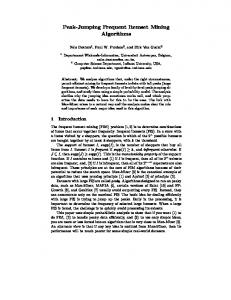
Figure 1. Structure of nodes on an AT-Tree

The node structure on an AT-Tree is illustrated in Figure 1. There are two types of nodes: one is normal node, as shown in Figure 1(a), where Name is the item name of each node; the other type is tail node, as shown in Figure 1(b), where Tail_info is the supplemental information that includes 4 fields: (1) bp: a list that keeps base probability values of all tail-node-itemsets; (2) len: the length of the tail-node-itemset; (3) Arr_ind: a list of index values of an array each element of which records probability values of items in each sorted transaction itemset (see Substep 5.2 in Section 4.2.1 and Step 5 in Section 4.2.2, etc.); (4) Item_ind: a list of index values of an array that records probability values of each item in a sorted transaction itemset (see Substep 10.5 and 10.7 in Section 4.3.2, etc., Item_ind is just used in a sub ATTree). B. Construction of an AT-Tree The structure of AT-Tree is designed to efficiently store the related information on tail nodes. It is constructed by two scans of dataset. In the first scan, a header table is created to maintain sorted frequent items.


In the second scan, the probability values of frequent items in each transaction itemsets are stored to a list according to the order of the header table; the list is then added to an array (and its corresponding sequence number in the array is denoted as ID); the frequent items in each transaction itemset are inserted to an AT-Tree according to the order of the header table; the length of the itemset and the number ID are stored to the corresponding tail node. When the transaction itemsets are added to an AT-Tree, they are rearranged in descending order of support numbers of items, and share the same node/nodes if their prefix items/itemsets are identical. Thus the AT-Tree is as compact as the original FP-Tree. Moreover, AT-Tree does not lose probability information with respect to the distinct probability values of the transaction itemsets. B.1 The construction algorithm of a global AT-Tree A global AT-Tree is the first AT-Tree that maintains itemset information of the whole dataset. The construction algorithm is described as follows: CreateTree(D, η ) INPUT: An uncertain database D consisting of n transaction itemsets and a predefined minimum expected support threshold η . OUTPUT: An AT-Tree T. Step 1: Calculate the minimum expected support number minExpSN, i.e. minExpSN =| D | ×η ; count the expected support number and support number of each item by one scan of dataset. Step 2: Put those items whose expected support numbers are not less than minExpSN to a header table, and sort the items in the header table according to the descending order of their support numbers; finish the algorithm if the header table is null. Step 3: Initially set the root node of the AT-Tree T as null. Step 4: Remove the items that are not in the header table from each transaction itemset, and sort the remaining items of each transaction itemset according to the order of the header table, and get a sorted itemset X. Step 5: If the length of itemset X is 0, process the next transaction itemset; otherwise insert the itemset X into the AT-Tree T by the following substeps: Substep 5.1: Store the probability value of each item in itemset X sequentially to a list; save the list to an array (which is denoted as ProArr); the corresponding sequence number of the list in the array is denoted as ID. Substep 5.2: If there has not been a tail node for the itemset X, create a tail node N for this itemset, where N.Tail_info.len is the length of itemset X, and N.Tail_info.Arr_ind={ID}; otherwise, append the sequence number ID to N.Tail_info.Arr_ind. Step 6: Process the next transaction itemset.


1421

“c” and a tail node “e”. The resulting AT-Tree is shown in Figure 2(c). Step 7: Process the next transaction T3, get the sorted transaction itemset {d:0.6, c:0.85, e:0.6}. Since the path “root-d-c-e” can be shared and the node “e” on the path is a tail node, just append the corresponding ID in ProArr of Table 2 to the Tail_info.Arr_ind of the tail node “e”. The resulting AT-Tree is shown in Figure 2(d). Step 8: Process the remaining transactions one by one. The resulting AT-Tree is shown in Figure 2(e). C. Mining Frequent Itemsets from a Global AT-Tree After an AT-Tree is constructed, the algorithm ATMine can directly mine frequent itemsets from the tree without additional scan of dataset. The details of the mining approach are described below. Figure 2. Construction of an AT-Tree

TABLE II. PROBABILITY LIST (PROARR)

ID 1 2 3 4 5 6

probabilities {0.9, 0.7, 0.8} {0.85, 0.8, 0.4} {0.6, 0.85, 0.6} {0.65, 0.85, 0.9} {0.8, 0.7, 0.95, 0.7} {0.7, 0.65}

B.2 An Example of Constructing a Global AT-Tree The uncertain dataset in Table 1 is used as an example here to illustrate the construction of the AT-Tree. This dataset concludes 6 transaction itemsets and 6 distinct items. The minimum support threshold is set as 20%. Step 1: Calculate the minimum expected support number as 1.2 (6*20%); count the expected support number and support number of each item by one scan of database. Step 2: Create a header table, as shown in Figure 2(a). Each link in the header table records all nodes of a corresponding item on a tree (not shown in the Figures for simplicity). Step 3: Initially set the root node of an AT-Tree as null. Step 4: Remove the infrequent item “f” from the transaction itemset T1, and sort the remaining items according to the order of the header table, the resulting is {d:0.9, b:0.7, a:0.8}. Step 5: Maintain probability value of each item to a list {0.9, 0.7, 0.8}, and append the list to an array ProArr, as shown in Table 2; the corresponding ID of the list in the array ProArr is 1; then insert the first sorted itemset into the AT-Tree, and the resulting AT-Tree is shown in Figure 2(b). On the tail node “a”, “3” represents the length of the tail-node-itemset (len), and “{1}” represents the index number of the array ProArr in Table 2.

Step 6: Process the next transaction T2, get the sorted transaction itemset {d:0.85, c:0.8, e:0.4}. Since the path “root-d” can be shared, insert a normal node © 2013 ACADEMY PUBLISHER

C.1 The Mining Algorithm The algorithm AT-Mine is similar to the algorithm FP-Growth: it creates and processes sub trees (prefix trees or conditional trees) recursively. But the condition of generating frequent itemsets is different from FPGrowth. The detailed steps of the mining algorithm are as follows: Mining (T, H, minExpSN) INPUT: An AT-Tree T, a header table H, and a minimum expected support number minExpSN. OUTPUT: The frequent itemsets (FIs). Step 1: Process the items in the header table one by one from the last item by the following steps (denote the currently processed item as Z). Step 2: Append item Z to the current base-itemset (which is initialized as null); each new base-itemset is a frequent itemset. Step 3: Let Z.links in the header table H contain k nodes whose item name is Z; we denote these k nodes as N1, N2, …, Nk; because item Z is the last one in the header table, all these k nodes are tail nodes, i.e., each of these nodes contains a Tail_info. Substep 3.1: Create a sub header table subH by scanning the k branches from these k nodes to the root. Substep 3.2: If the sub header table is null, go to Step 4. Substep 3.3: Create sub AT-Tree subTree = CreateSubTree(Z.link, subH). Substep 3.4: Mining(subTree, subH, minExpSN). Step 4: Remove item Z from the base-itemset. Step 5: For each of these k nodes (which we denote as Ni, 1≤i≤k), modify its Tail_info by the following substeps: Substep 5.1: Alter Ni.Tail_info.len values: Ni.Tail_info.len = Ni.Tail_info.len -1. Substep 5.2: Move Ni.Tail_info to the parent of node Ni. Step 6: Process the next item of the header table H. Subroutine: CreateSubTree(link, subH) INPUT: A list link which records tree nodes with the same item name, and a header table subH. OUTPUT: An AT-Tree subT.

1422

Step 1: Initially set the root node of the tree subT as null. Step 2: Process each node in the list link by the following steps (denote the currently processed node as N). Step 3: Get the tail-node-itemset of node N (denote it as itemset X). Step 4: Remove those items that are not in the header table subH from itemset X, and sort the remaining items in itemset X according to the order of the header table subH. Step 5: If the length of the sorted itemset (denoted as k) is 0, process the next node of the list link; otherwise insert the sorted itemset X into the AT-Tree subT by the following substeps: Substep 5.1: Get the original sequential ID of each item of the itemset X in the corresponding list of ProArr: item_ind = {d1, d2, .., dk} (k is the length of itemset X). Substep 5.2: Make a copy of N.Tail_info; denote the copy as nTail_info. Substep 5.3: Alter nTail_info as the following: (1) nTail_info.len = k. (2) nTail_info. Item_ind = item_ind. (3) if nTail_info.bp is null, set nTail_info.bp[j] to be the probability of item Z, i.e. ProArr[nTail_info.Arr_ind[j]]; otherwise, set nTail_info.bp[j] to be the product of nTail_info.bp[j] and the probability of item Z (1 ≤ j ≤ bp.size; the array ProArr is created when the global tree is created in Substep 5.1 in Section 4.2.1). C.2 An Example of Mining Frequent Itemsets from a Global AT-Tree

Figure 3. An Example of mining frequent itemsets from uncertain dataset

The global AT-Tree in Figure 2(e) and its corresponding header table H in Figure 2(a) are used as an example here to illustrate the detailed processes of mining frequent itemsets. The minimum expected support number is 1.2. Step 1: Process the item “e” in the header table H by the following steps 2-3. Step 2: Append item “e” to the current base-itemset (which is initialized as null), and generates a new frequent itemset {e}. Step 3: Scan the branches containing the node “e” to create sub header table: Substep 3.1: In Figure 2(e), there are 2 nodes “e”. From the path “root-d-b-a-e” and Table 2, the expected support numbers of itemsets {ed}, {eb} © 2013 ACADEMY PUBLISHER


and {ea} are calculated as 0.56 (0.7*0.8), 0.49 (0.7*0.7) and 0.665 (0.7*0.95), respectively; from the path “root-d-c-e”, the expected supports of itemset {ed} and {ec} are calculated as 0.7 (0.4*0.85+0.6*0.6) and 0.83 (0.4*0.8+0.6*0.85). Substep 3.2: Because the total expected support numbers of itemset {ed} is bigger than 1.2, the sub header table is not null, create a sub tree (prefix tree or conditional tree) for the baseitemset {e}, and get a new frequent itemset {ed}. SubStep 3.3: Remove the item “e” from the baseitemset, pass the Tail_info of nodes “e” to their parents, and modify Tail_info.len as Tail_info.len -1; the result is shown in Figure 3(a). Step 4: Process the next item “c” in the header table H by the following steps 5-6. Step 5: Append item “c” to base-itemset, and get a new frequent itemset {c}. Step 6: Scan the branches containing node “c” to create the sub header table: Substep 6.1: In Figure 3(a), there are 2 nodes “c”. From the path “root-d-c” and Table 2, the expected support numbers of itemset {cd} is calculated as 1.19 (0.8*0.85+0.85*0.6); from the path “root-b-c”, the expected support of itemset {cb} is calculated as 0.455 (0.65*0.7). Substep 6.2: Because the total expected support numbers of itemsets {cd} and {cb} are smaller than 1.2, the sub header table is null. SubStep 6.3: Remove the item “c” from the baseitemset, pass the Tail_info of nodes “c” to their parents; the result is shown in Figure 3(b). Step 7: Process the next item “a” in the header table in Figure 2(a) as the following steps 8-10. Step 8: Append item “a” to the base-itemset, and get a new frequent itemset {a}. Step 9: Scan the branches containing node “a” to create the sub header table: Substep 9.1: In Figure 3(b), there is one node “a”. From the path “root-d-b-a” and Table 2, the expected support numbers of itemsets {ad} and {ab} are calculated as 2.065 (0.8*0.9+0.9*0.65+0.95*0.8) and 1.99 (0.8*0.7+0.9*0.85+0.95*0.7). Substep 9.2: Because the total expected support numbers of itemsets {ad} and {ab} are not smaller than 1.2, the sub header table subH is {d:2.065:3, b:1.99:3}. Step 10: Create a sub tree for the base-itemset {a} by the following substeps: Substep 10.1: Initially set the root node of the sub tree subT as null. Substep 10.2: Get the itemset {db} from the tailnode-itemset of the tail node “a” in Figure 3(b). Substep 10.3: Sort the itemset {db} in the order of the header table subH. Substep 10.4: Make a copy of Tail_info.Arr_ind,


1423

and denote it as arr_ind={1, 4, 5}. Substep 10.5: Get the list indexes (original sequential ID in a list) of items “d” and “b” in the list ProArr[1], which are 1 and 2 respectively, and denote it as item_ind={1, 2}. Substep 10.6: Get the probability values of itemset {a} in ProArr[1] and ProArr[4] and ProArr[5] respectively, and denote them as bp={0.8, 0.9, 0.95}; this is the corresponding base probabilities in the sub tree subT. Substep 10.7: Add the sorted itemset {db} to subT; maintain arr_ind, item_ind, bp and the length of the itemset {db} to the tail node in subT; the result is shown in Figure 3(c). Substep 10.8: Process the tree subT recursively, and get a new sub tree for the base-itemset {ab}, as shown in Figure 3(d). Lastly, get frequent itemsets {ab}, {abd} and {ad} when processing the sub tree of itemset {a}. Step 11: Go on processing the remaining items in header table H.

transaction itemset; as suggested by literatures [23, 25, 28, 29], we assign a existential probability of range (0, 1] to each item. The runnable programs and testing datasets can be downloaded from the following address: http://code.google.com/p/at-tree/downloads/list. A. Evaluation on Sparse Datasets Tables 4-5 show the total number of tree nodes generated by AT-Mine, UF-Growth and CUFP, and the number of candidate itemsets generated by MBP, respectively, on the sparse datasets. As shown in Tables 4-5, UF-Growth creates much more tree nodes than ATMine. This is because that UF-Growth just merges the nodes that have the same item name and the same probability. CUFP-Mine is out of memory on these two sparse datasets because it generates too many supersets; UF-Growth is out of memory on kosarak when the threshold is set 0.01% because it generates too many tree nodes; MBP is out of memory when the threshold is set 0.03% because it generates too many candidates. Thus we can infer that AT-Mine has a better performance than other three algorithms in terms of memory usage.

V. EXPERIMENTAL RESULTS In this section, we evaluate the performance of the proposed algorithm AT-Mine. Summarizing the related works in Section 3, we can conclude that the algorithm MBP is the state-of-the-art algorithm employing the level-wise approach, UPGrowth is the state-of-the-art algorithm employing the pattern-growth approach and CUFP-Mine is a new proposed algorithm. So we compare AT-Mine with the algorithms UF-Growth, CUFP-Mine and MBP on both types of datasets: the sparse transaction datasets and dense transaction datasets. All algorithms were written in Java programming language. The configuration of the testing platform is as follows: Windows XP operating system, 2G Memory, Intel(R) Core(TM) i3-2310 CPU @ 2.10 GHz; Java heap size is 1G.

TABLE IV. DETAILS ANALYSIS ON THE DATASET T20I6D300K

trees nodes (#)

η (%)

AT-Mine 4,978,327 5,101,077 5,438,410 6,310,746 8,474,124 13,189,900

0.15 0.13 0.11 0.09 0.07 0.05

Dataset T20I6D 300K kosarak connect mushroom

|D|

|I|

ML

SD (%)

Type

300,000

1000

20

2

sparse

990,002 67,557 8,124

41,271 129 119

8 43 23

0.02 33.33 19.33

sparse dense dense

UF-Growth 7,556,250 8,629,034 10,282,811 12,978,032 17,477,552 24,946,139

MBP 374,271 391,413 419,770 467,217 594,050 999,799

TABLE V. DETAILS ANALYSIS ON THE DATASET KOSARAK

trees nodes (#)

η (%) TABLE III. DATASET CHARACTERISTICS

candidates (#)

0.1 0.09 0.07 0.05 0.03

AT-Mine 2,020,568 2,208,231 2,542,835 3,058,380 4,580,785

0.01

18,829,877

candidates (#)

UF-Growth 14,471,137 15,724,272 19,210,453 24,651,644 38,083,667 Memory Overflow

MBP 172,399 252,348 419,272 793,554 Memory Overflow

10000


AT-Mine MBP UF-Growth CUFP-Mine (Memory Overflow) Running time (s)

Table 3 shows the characteristics of 4 datasets used in our experiments. “|D|” represents the total number of transactions; “|I|” represents the total number of distinct items; “ML” represents the mean length of all transaction itemsets; “SD” represents the degree of sparsity or density. The synthetic dataset T20I6D300K came from the IBM Data Generator [1] and the datasets kosarak, connect and mushroom were obtained from FIMI Repository [33]; These four datasets originally do not provide probability values for each item of each

1000

100

10 0.15

0.14

0.13

0.12

0.11

0.10

0.09

0.08

0.07

Minimum expected support threshold (%)

0.06

0.05

1424


TABLE VII. DETAILS ANALYSIS ON THE DATASET MUSHROOM

AT-Mine MBP UF-Growth CUFP-Mine (Memory Overflow)

1000

Running time (s)

On the dataset T20I6D300K

100

10 0.10

0.09

0.08

0.07

0.06

0.05

0.04

0.03

0.02

0.01


(b)

Figure 4 shows the running time of three algorithms on two sparse datasets. CUFP-Mine is out of memory on these two sparse datasets. As shown in Figure 4, the time performance of our algorithm outperforms UF-Growth, MBP and CUFP-Mine under different minimum expected support thresholds. This is because that CUFP-Mine generates too many supersets and UF-Growth generates too many tree nodes and MBP generates many candidates, as shown in Tables 4-5. The time performance of MBP is dependent on the length of candidate itemsets, the length of transaction itemsets, and the size of dataset: the higher these values are, the lower the time performance of MBP will be. Thus the time performance of MBP decreases sharply with the decreasing of the threshold. Figure 4 indicates that AT-Mine has achieved a better time performance; moreover, its time performance is more stable on sparse dataset. B. Evaluation on Dense Datasets In this section, we test the performance of our proposed algorithm on dense datasets connect and mushroom. TABLE VI. DETAILS ANALYSIS ON THE DATASET CONNECT

15.0 14.0 13.0 12.0 11.0 10.0

7.0 6.0 5.0 4.0 3.0 2.0

candidates(#) MBP 1,917 2,501 3,460 5,024 8,222 16,764

On the dataset kosarak

Figure 4. Running time comparison on sparse datasets

η (%)

trees nodes (#) AT-Mine UF-Growth 12,041 1,011,721 14,420 1,344,369 16,243 1,947,609 18,685 2,760,249 25,884 4,125,745 37,395 8,076,099

η (%)

trees nodes (#) AT-Mine UF-Growth 36,823 32,204,274 89,118 33,739,243 98,842 35,332,360 116,290 48,046,639 130,423 106,626,725 153,913 163,809,762

candidates (#) MBP 5,981 6,962 7,786 8,565 12,754 19,162

Tables 6-7 show the total number of tree nodes generated by AT-Mine and UF-Growth, and the number of candidate itemsets generated by MBP, on the dense datasets. As shown in Tables 6-7, UF-Growth creates too many tree nodes. For example, on the dataset connect, UF-Growth generates 163,809,762 nodes while AT-Mine generates 153,913 nodes when the minimum expected support threshold is 10%. This is because that UFGrowth just merges the nodes that have the same item name as well as the same probability, and it is a very dense and long dataset. Thus we can infer that our algorithm has achieved better performance than UFGrowth in terms of memory usage. MBP not only maintains candidates, but also maintain the dataset while our algorithms only maintain tree nodes using compact trees. Figure 5 shows the running time of three algorithms on the dense datasets connect and mushroom. CUFPMine is out of memory on these two dense datasets. As shown in Figure 5, the time performance of our algorithm prevails over UF-Growth, MBP and CUFP-Mine under different minimum expected support thresholds. This is because that CUFP-Mine generates too many supersets and UF-Growth generates too many tree nodes and MBP generates many candidates, as shown in Tables 6-7. Figure 5 shows that the time performance of AT-Mine obviously outperforms that of other algorithms on these two dense datasets; moreover, our time performance is also more stable on the dense datasets. 10000

Running time (s)

(a)


1000

100

10 15.0

14.5

14.0

13.5

13.0

12.5

12.0

11.5

11.0

10.5


(a)


On the dataset connect

10.0



60

50

Running time (s)

40

30

20

10

0 7.0

6.5

6.0

5.5

5.0

4.5

4.0

3.5

3.0

2.5

2.0


(b)

On the dataset mushroom

Figure 5. Running time comparison on dense datasets

VI. CONCLUSION AND DISCUSSION In this paper, we propose a novel tree structure named AT-Tree to maintain transaction itemsets of an uncertain dataset, and a corresponding algorithm named AT-Mine to mine frequent itemsets. AT-Mine requires two scans of dataset to create an AT-Tree. In the first scan, it creates a header table to maintain sorted frequent items in the descending order of support numbers of items. In the second scan, it maintains probability values of frequent items in each transaction itemsets to an array; it inserts frequent items in each transaction itemsets to an AT-Tree; it maintains probability information of each transaction itemsets to the tail node. So the AT-Tree is as compact as the original FP-Tree, and it does not lose the probability information of each transaction itemsets. Thus, AT-Mine can find frequent itemsets from AT-Tree without additional scan of dataset. Experiments were performed on sparse and dense datasets. We compared our proposed algorithm with some state-of-the-art level-wise and pattern-growth algorithms. The experimental results show that the proposed algorithm has better performance on dense datasets and large sparse datasets, and their time performance is stable on both dense and sparse datasets along with the decreasing of the minimum expected support threshold. REFERENCES [1] R. AGrawal and R. Srikant, Fast algorithms for mining association rules in large databases, in International Conference on Very Large Data Bases. 1994, pp.487-487. [2] J. Han, J. Pei and Y. Yin, Mining frequent patterns without candidate generation, in ACM SIGMOD International Conference on Management of Data. 2000, pp.1-12. [3] G. Grahne and J. Zhu, "Fast algorithms for frequent itemset mining using FP-trees," IEEE Transactions on Knowledge and Data Engineering, Vol.17, no.10, pp.1347-1362, 2005. [4] M. Song and S. Rajasekaran, "A transaction mapping algorithm for frequent itemsets mining," IEEE Transactions on Knowledge and Data Engineering, Vol.18, no.4, pp.472-481, 2006. [5] J. Pei, et al., "H-Mine: Fast and space-preserving frequent pattern mining in a large databases," IIE Transactions (Institute of Industrial Engineers), Vol.39, no.6, pp.593605, 2007. [6] P. Paranjape-Voditel and U. Deshpande, "A DIC-based


1425

distributed algorithm for frequent itemset generation," Journal of Software, Vol.6, no.2, pp.306-313, 2011. [7] L. Zhou and Z. Zhang, "Efficient mining algorithms of finding frequent datasets," Journal of Software, Vol.7, no.4, pp.727-732, 2012. [8] R.C. Agarwal, C.C. Aggarwal and V.V.V. Prasad, Depth first generation of long patterns, in ACM SIGKDD International Conference on Knowledge Discovery and Data Mining. 2001, pp.108-118. [9] R.J. Bayardo Jr., Efficiently mining long patterns from databases, in ACM SIGMOD International Conference on Management of Data. 1998, pp.85-93. [10] D. Burdick, M. Calimlim, J. Flannick, J. Gehrke, and T. Yiu, "MAFIA: A maximal frequent itemset algorithm," IEEE Transactions on Knowledge and Data Engineering, Vol.17, no.11, pp.1490-1504, 2005. [11] D.I. Lin and Z.M. Kedem, "Pincer search: A new algorithm for discovering the maximum frequent set," IEEE Transactions on Knowledge and Data Engineering, Vol.3, no.14, pp.553- 566, 2002. [12] H. Li, N. Zhang and Z. Chen, "A simple but effective maximal frequent itemset mining algorithm over streams," Journal of Software, Vol.7, no.1, pp.25-32, 2012. [13] J. Wang, J. Han and J. Pei, CLOSET+: Searching for the best strategies for mining frequent closed itemsets, in ACM SIGKDD International Conference on Knowledge Discovery and Data Mining (KDD '03). 2003, pp.236-245. [14] B. Vo, T. Hong and B. Le, "DBV-Miner: A Dynamic BitVector approach for fast mining frequent closed itemsets," Expert Systems with Applications, Vol.39, no.8, pp.71967206, 2012. [15] J. Wang, J. Han, Y. Lu, and P. Tzvetkov, "TFP: An efficient algorithm for mining top-k frequent closed itemsets," IEEE Transactions on Knowledge and Data Engineering, Vol.17, no.5, pp.652-664, 2005. [16] C.H. Wei and R. Gob, "Discovering patterns in categorical time series using IFS," Computational Statistics and Data Analysis, Vol.52, no.9, pp.4369-4379, 2008. [17] J.Y. Hu and A.M. Silovic, "High-utility pattern mining: A method for discovery of high-utility item sets," PATTERN RECOGNITION, Vol.40, no.11, pp.3317-3324, 2007. [18] C.F. Ahmed, S.K. Tanbeer, B.S. Jeong, and Y.K. Lee, "Efficient Tree Structures for High Utility Pattern Mining in Incremental Databases," IEEE Transactions on Knowledge and Data Engineering, Vol.21, no.12, pp.17081721, 2009. [19] V.S. Tseng, C.W. Wu, B.E. Shie, and P.S. Yu. UP-Growth: An efficient algorithm for high utility itemset mining, in ACM SIGKDD International Conference on Knowledge Discovery and Data Mining. 2010, pp.253-262. [20] V.S. Tseng, B. Shie, C. Wu, and P.S. Yu, "Efficient Algorithms for Mining High Utility Itemsets from Transactional Databases," IEEE Transactions on Knowledge and Data Engineering, no.99(PrePrints), 2012. [21] A. Prasad Sistla, O. Wolfson, S. Chamberlain, and S. Dao, "Querying the uncertain position of moving objects," Vol.1399, pp.310-337, 1998. [22] N. Khoussainova, M. Balazinska and D. Suciu, Towards correcting input data errors probabilistically using integrity constraints, in MobiDE 2006: 5th ACM International Workshop on Data Engineering for Wireless and Mobile Access. 2006, pp.43-50. [23] C.W. Lin and T.P. Hong, "A new mining approach for uncertain databases using CUFP trees," Expert Systems with Applications, Vol.39(4), pp.4084–4093, 2012. [24] C.C. Aggarwal and P.S. Yu, "A survey of uncertain data algorithms and applications," Knowledge and Data

1426

Engineering, IEEE Transactions on, Vol.21, no.5, pp.609623, 2009. [25] C.K. Leung, M.A.F. Mateo and D.A. Brajczuk, A treebased approach for frequent pattern mining from uncertain data, in 12th Pacific-Asia Conference on Knowledge Discovery and Data Mining (PAKDD 2008). 2008, pp.653661. [26] X. Sun, L. Lim and S. Wang, "An approximation algorithm of mining frequent itemsets from uncertain dataset," International Journal of Advancements in Computing Technology, Vol.4, no.3, pp.42-49, 2012. [27] T. Calders, C. Garboni and B. Goethals, Approximation of frequentness probability of itemsets in uncertain data, in IEEE International Conference on Data Mining (ICDM 2010). 2010, pp.749-754. [28] L. Wang, D.W. Cheung, R. Cheng, S. Lee, and X. Yang, "Efficient Mining of Frequent Itemsets on Large Uncertain Databases," IEEE Transactions on Knowledge and Data Engineering, no.99(PrePrints), 2011. [29] C.K. Leung, C.L. Carmichael and B. Hao, Efficient mining of frequent patterns from uncertain data, in International Conference on Data Mining Workshops (ICDM Workshops 2007). 2007, pp.489-494. [30] C.C. Aggarwal, Y. Li, J. Wang, and J. Wang, Frequent pattern mining with uncertain data, in 15th ACM SIGKDD International Conference on Knowledge Discovery and Data Mining (KDD '09). 2009, pp.29-37. [31] C. Chui, B. Kao and E. Hung, Mining frequent itemsets from uncertain data, in 11th Pacific-Asia Conference on Knowledge Discovery and Data Mining (PAKDD 2007). 2007, pp.47-58. [32] Y. Liu, "Mining frequent patterns from univariate uncertain data," Data and Knowledge Engineering, Vol.71, no.1, pp.47-68, 2012. [33] B. Goethals. Frequent itemset mining dataset repository, http://fimi.cs.helsinki.fi/data/. Accessed June 2011,2011.

