E. Bemis,. â . S. Hough,. â and K. Zaleski. â . North Carolina State University, Hampton, Virginia ... George Washington University, Newport News, Virginia 23606.
JOURNAL OF SPACECRAFT AND ROCKETS Vol. 45, No. 3, May–June 2008
Atmospheric Modeling Using Accelerometer Data During Mars Reconnaissance Orbiter Aerobraking Operations R. Tolson,∗ E. Bemis,† S. Hough,† and K. Zaleski† North Carolina State University, Hampton, Virginia 23666 G. Keating‡ George Washington University, Newport News, Virginia 23606 and J. Shidner,† S. Brown,† A. Brickler,† M. Scher,† and P. Thomas† University of Maryland, Hampton, Virginia 23666 DOI: 10.2514/1.34301 Aerobraking as an enabling technology for the Mars Reconnaissance Orbiter mission was used in numerous analyses based on various data types to maintain the aerobraking time line. Among these data types were measurements from spacecraft accelerometers. This paper reports on the use of accelerometer data for determining atmospheric density during Mars Reconnaissance Orbiter aerobraking operations. Acceleration was measured along three orthogonal axes, although only data from the component along the axis nominally into the flow were used during operations. For a 1-s count time, the root-mean-square noise level was 0:004 mm=s2 , permitting density recovery to 0:008 kg=km3 , or about 0.023% of the mean density at periapsis, during aerobraking. Accelerometer data were analyzed in near real time to provide estimates of density, density scale height, orbit-to-orbit variability, latitudinal-seasonal variations, longitudinal waves, and other phenomena in the thermosphere. Summaries are given of the aerobraking phase of the mission, the accelerometer data analysis methods and operational procedures, some applications to determining thermospheric properties, correlation with the Mars Global Surveyor and Odyssey missions, and some remaining issues on interpretation of the data.
70 days. During Magellan, adjustments were made to the Venus atmospheric model based on orbital decay drag data. The second application began in September 1997 when over 850 Mars Global Surveyor (MGS) aerobraking passes were used to reduce the postMars-orbit-insertion (MOI) period from about 45 h to about 2 h, saving an equivalent impulsive Delta-V (DV) of approximately 1200 m=s [2]. MGS was the first planetary mission in which aerobraking was essential for mission success. A second aerobraking mission followed in 2001, using over 300 Mars Odyssey (ODY) aerobraking passes to reduce the post-MOI period of 18 h to an MGS similar 2-h period, saving an equivalent impulsive DV of approximately 1100 m=s [3]. Although the Venusian atmosphere demonstrated less than 10% 1-� orbit-to-orbit variability in density, the Mars atmosphere demonstrated between 30 to 50%. During MGS and ODY, persistent density waves were found to exist in the equatorial region that could produce nearly a factor-of-2 change in density from trough to peak. Further, a regional dust storm in the southern hemisphere produced over a factor-of-2 increase in density at the periapsis latitude of 60� N during MGS aerobraking [4]. The primary drag surfaces for Magellan, MGS, ODY, and the Mars Reconnaissance Orbiter (MRO) were the solar arrays. Solar array temperatures were the preaerobraking criteria limiting the pace of aerobraking. Because of the damaged solar array, MGS aerobraking was actually limited by maximum dynamic pressure during each pass at about one-half of the heating limit . The large systematic atmospheric variations discovered and confirmed during MGS and ODY were not as large of a concern for MRO, because the design could tolerate up to a 250% margin on the solar panel thermal limits. Nevertheless, the mission failure of the MGS solar panel leads to numerous additional atmospheric modeling activities [5], mission simulations [6], and thermal analyses [7] before MOI for MRO.
Nomenclature A a Cy Hs h ho Ls m Nq r ux uz V � !
= = = = = = = = = = = = = = =
aerodynamic reference area, m2 acceleration, m=s2 y-axis aerodynamic force coefficient density scale height, km geodetic altitude, km geodetic reference altitude, km celestial longitude of Mars, deg Mars Reconnaissance Orbiter mass, kg Nyquist, samples per second accelerometer position in the body system, m x-axis component of the relative wind unit vector z-axis component of the relative wind unit vector spacecraft speed relative to the atmosphere, km=s atmospheric density, kg=km3 body angular rate, rad=s
Introduction
A
EROBRAKING is the use of atmospheric drag for beneficial orbit changes via multiple passes through an atmosphere. The first application of aerobraking in a planetary mission was during the Magellan mission at Venus [1]. To increase imaging radar and gravity field resolution in the polar region, aerobraking was performed during the extended mission in 1993 over about 750 orbital passes to reduce the eccentricity from 0.3 to 0.03 in about
Presented as Paper AAS-07-183 at the 17th Annual AAS/AIAA Space Flight Mechanics Meeting, Sedona, AZ, 28 January–1 February 2007; received 28 August 2007; revision received 9 January 2008; accepted for publication 2 January 2008. Copyright © 2008 by the American Institute of Aeronautics and Astronautics, Inc. All rights reserved. Copies of this paper may be made for personal or internal use, on condition that the copier pay the $10.00 per-copy fee to the Copyright Clearance Center, Inc., 222 Rosewood Drive, Danvers, MA 01923; include the code 0022-4650/08 $10.00 in correspondence with the CCC. ∗ Professor. Associate Fellow AIAA. † Graduate Research Scholar Assistant. ‡ Senior Research Staff Scientist. Associate Fellow AIAA.
MRO Aerobraking Mission Summary The aerobraking configuration is shown in Fig. 1. Though not shown here, the bus is surrounded by thermal insulation. This configuration provides strong aerodynamic stability about the body z and x axes, where z nominally points toward the center of Mars and x 511
512
TOLSON ET AL.
Fig. 1 Mars Reconnaissance Orbiter spacecraft in an aerobraking configuration, without thermal blankets.
is nominally horizontal during aerobraking. The spacecraft (s/c) is almost neutrally stable about the y axis, which is along the velocity direction and normal to the plane of the solar array. Active damping using eight reaction control system thrusters is therefore used to maintain control about the y axis and to limit angular rates and excursions about the other two axes. The y axis is within 5.5 deg of the aerodynamic trim direction. The photovoltaic cells are oriented away from the flow to minimize solar cell heating. After MOI on 10 March 2006, the orbital period was 35 h, and the goal of aerobraking was to reduce the period to 2 h by about 30 August 2006. The reference period decay profile, developed just after MOI, is shown in Fig. 2. Also shown is the actual orbital period achieved during aerobraking. The difference between the reference and actual trajectory at the end is indirectly due to the reference trajectory changing the initial target for the ascending node of 3:15 p.m. LMST (local mean solar time). As the mission progressed, the arrival conditions were retargeted, instead arriving at an ascending node of 3:10 p.m. LMST and an orbital period less than the initially targeted orbital period. The first few orbits were spent checking s/c systems before the periapsis altitude was dropped into the sensible atmosphere. The “walk-in” phase began with orbit 18 measuring an atmospheric density of 0:054 kg=km3 at a 148-km altitude. Orbits 24–34 began the main aerobraking phase with periapsis altitudes around 108 km and densities ranging from 12 to 30 kg=km3 . Variations in density were not as large as seen in MGS and ODY during walk-in; however, MRO periapsis was already south of 70� S, well within the estimated location of the Mars polar vortex. At the time of walk-in, the polar vortex was estimated to be around 65� S. While inside the vortex, the orbit-to-orbit variability in density was low and aerobraking could be performed with greater confidence. On ODY, reduced variability was also found inside the polar vortex [3]. Once the MRO periapsis began precessing toward the equator, the increased variability in the density reduced the accuracy of the orbit-to-orbit density predictions. After 147 days, aerobraking ended on 30 August 2006. The MRO final science orbit
is a near-polar 255 � 320 km orbit with an ascending node at 3:00 p.m. LMST [8]. Orbital characteristics of interest for aerobraking are shown in Fig. 3 for the entire aerobraking phase. The figure presents geodetic altitude, latitude, local solar time (LST), and Ls at periapsis. Ls is the celestial longitude of Mars measured from the Mars vernal equinox and is a measure of Mars season and distance from the sun. These four variables are the most significant in determining thermospheric mean properties. The altitude plot shows walk-in (orbits 18–23); main phase, in which solar array temperature was the limiting factor (orbits 24 to 428); and walk-out, in which orbital lifetime was the limiting factor (orbits 429–445). Orbit-to-orbit periapsis-altitude variations of 1 to 2 km are due to high-order gravity field terms. Precession of the line of apsides due to planetary oblateness (J2 ) moved periapsis poleward for the first 143 orbits and then toward the equator through the end of the mission. Geodetic altitude is of interest because in a static atmosphere, equal pressure surfaces would be equipotential surfaces. Up to the time of maximum latitude, the J3 long-period variation in eccentricity causes periapsis altitude to increase with time. Likewise, as the periapsis precesses southward due to J2 , the flattening of the planet causes geodetic altitude to increase. Both effects reverse after the time of maximum latitude. These two effects are the same order of magnitude and provided a fail-safe situation early in the mission. It is clear that after orbit 180, these two effects continued to drive periapsis lower into the atmosphere, and many maneuvers were performed to keep the altitude in the aerobraking corridor. The general trends are primarily due to the latitudinal density gradient, which, at a constant geodetic altitude, causes density to decrease toward the colder pole. Contrary to past missions, the walk-out phase required maneuvers that lowered the periapsis altitude so that aerobraking would remain in the desired corridor during walk-out. Local solar time, as for all nearHohmann transfers to outer planets, starts near 20:00 hrs. Because nodal regression is essentially zero for this nearly polar orbit, LST initially becomes earlier due to Mars orbital motion. Eventually, northward apsidal precession combined with Mars obliquity begins to dominate and LST moves into night and rapidly shifts to morning hours as periapsis passes over the pole. The aerobraking mission lasted less than two Mars months, and so the season at Mars remained in southern hemisphere fall (0 < Ls < 90) throughout aerobraking.
Atmospheric Density Recovery Because the y component provides the largest acceleration signalto-noise ratio (Fig. 1), it was used to recover atmospheric density. The density recovery is based on Newton’s second law and the definition of aerodynamic coefficients: may �
�V 2 Cy A 2
(1)
25 20
105 100 200
400
200 300 Orbit Number
400
500
Planned and actual orbital periods during aerobraking.
−60
0
200
400
20
200
0 0
100
−40
−80 95 0
100
5
Fig. 2
110
LST, hours
10
0 0
0 −20
300
15 Ls, deg
Orbital Period, hours
30
115 Latitude, deg
Ref Traj: 03/20/06 Actual Trajectory
35
Geodetic Altitude, km
40
200 400 Orbit number
Fig. 3 Variables of interest for Reconnaissance Orbiter mission.
15 10 5 0 0
200 400 Orbit number
aerobraking
for
the
Mars
513
TOLSON ET AL.
To use acceleration measurements to determine atmospheric density from Eq. (1), an aerodynamic database of Cy is required that covers the s/c operational range. The knowledge in the aerodynamic coefficient is assumed to be perfect for the results presented; however, the aerodynamics have an operational uncertainty of 4.5% as defined by the creators of the database. Main-phase aerobraking was to take place at a nominal heat flux of about 0:11 W=cm2 , which corresponded to an atmospheric density of about 24 kg=km3 . Aerodynamic coefficients were generated for 14 values of � up to 350:05 kg=km3 . Aerodynamic properties were calculated with direct simulation Monte Carlo (DSMC) and free-molecular flow codes [7]. The DSMC method was required to accurately quantify aerothermodynamics in the regions of highest dynamic pressure. DSMC and free-molecular simulations were performed over heading angles up to 30 deg. The force coefficient over the range of expected densities for flow along the y axis is shown on the right in Fig. 4. The value at � � 0:001 is the free-molecular flow value, and this value is used for lower densities. All calculations are based on assumed momentum accommodation coefficients of unity. The highest density encountered during aerobraking was on orbit 262 with a value of 86:4 kg=km3 . Contours of Cy variation with wind direction are shown on the right in Fig. 4 for a density of 100 kg=km3 . The variables ux and uz are the components of the relative wind unit vector in the s/c body coordinates shown in Fig. 1. In recovering density from accelerometer data, the aerodynamic database is used as a function of the density and relative wind unit vector to solve Eq. (1) in an iterative manner. The relative wind unit vector (ux or uz ) is determined from the attitude quaternions and the orbital ephemeris assuming a rigidly rotating atmosphere with the planet. The initial guess of density is determined using Cy equal to 2 in Eq. (1). For each accelerometer measurement, the previous value of density is used to interpolate into the aerodynamic database to update the Cy estimate, and the process continues until density converges to within 0.1% relative change of the previous value. Inertial Measurement Unit Data
Two inertial measurement units (IMUs) are located on the middeck of the s/c, as shown in Fig. 1. The primary IMU was used throughout aerobraking. Although the IMUs used on MRO were the same as ODY (QA-2000 accelerometers and GG1320 Ring Laser Gyros), a substantial improvement to the accelerometer electronics was performed at Honeywell. This improvement reduced readout noise in the accelerometers by approximately 36x, 16x, and 10x in the x, y, and z axes. The accelerometer range of measurement was reduced from ODY levels of �35 to �1:86 g. Bias stability for the accelerometers is less than 100 �g over a 4-h time period, and the scale factor error is less than 240 ppm over a 1-year time period. The principle acceleration used in the aerobraking analysis is the y direction. The accelerometers are located at r � �0:851, � 1:630, and �0:575 m relative to the center of mass in the spacecraft’s mechanical frame. The accelerometers and gyros were sampled at 200 Nyquist samples per second (Nq). The accelerometer output was quantized at 0:0753 �mm=s�=count. The gyro output was quantized −1.7
0
3
10 10 10 3 Density, kg / km
−1.3
.3
−1.5
0
−1.5
−1 .
9
−0.4 −0.2
a m � ab � aa � ag � aACS � ! � �! � r� � !_ � r
0.2 0.4
uz
Fig. 4 Y-axis force coefficient over a range of atmospheric density for ux � uz � 0 vs relative wind direction for � � 100 kg=km3 .
(2)
where the terms are, respectively, acceleration due to the instrument bias, aerodynamic forces, gravity gradient (negligible), attitude control system thruster activity (ACS), and angular motion of the accelerometer about the center of mass (two terms). The gyro rate data used were not altered or filtered from the given ground-averaged values. To illustrate the density recovery process, orbit 146 was selected. This orbit provides acceleration variations that are somewhat similar to the classical bell curve and also demonstrates some of the local variations during a pass. The raw accelerometer data along the y axis, from which density was derived, is shown in Fig. 5. As previously described, in the derivation of density, the process simultaneously recovers the Cy coefficient. The value of Cy for this pass is shown in the lower left. The Cy value is flat during the first 200 s, indicating alignment of the y axis with the wind in the aerobraking configuration, then increases about 5% during the 150 s before periapsis, primarily due to the transition flow phenomena shown in Fig. 4. On the outbound portion of the pass, Cy returns to the freemolecular value just before 200 s. Accelerometer bias was calibrated on the s/c by averaging measurements before encountering the atmosphere and after leaving the atmosphere. This constant value was automatically subtracted from the measurements in the flight data system before the 1-s averaging was done. Subsequent analysis showed that the bias was different between the inbound and outbound legs of a pass, probably due to the general increase in temperature of the IMU throughout a pass. During operations, a linear time-dependent bias was determined using inbound and outbound data. Through the pass, this model was evaluated at each observation time. An example of the process is shown in Fig. 6. The light gray x marks show the 1-saveraged acceleration data from the flight data system. The dark gray line is the seven-point running mean. To determine the bias, inbound and outbound data were selected visually, as indicated by the black � and ○ marks, and a least-squares fit is used to obtain the linear model. The data in the window selected typically contained outliers due to errors in the angular bias and thruster firings. To remove these outliers, a selection to omit data above 2 to 3.5 standard deviations was made by the analyst as seen by the ○ marks. The linear bias was then fit to the reduced data. Three values of the least-squares fit are shown along the top part of the figure, and the mean and standard deviation of the data points are shown on the bottom part of the
2
x 10
−3
0 −2 −4 −6
Cy −1.95 −2
−8
−2.05
−10 −2.1
−12 −400 −200
−1
−1.5 −1.7
y
C
ux −3
−1.7
.3 −1
−0.4 −2.3
−1.5
−0.2
.9 −1
0
−1.3
−2
−1.7 −1.5 −1.7
0.2
.3 −1
−1.5
0.4
at 0:001 mrad=count. For the purposes of density recovery, the high rate data were averaged over 1-s intervals. Throughout aerobraking, all data recorded on the s/c at 200 Nq were transmitted to the ground and averaged. The measured acceleration is composed of a number of terms given by
1 second y acceleration, m/s 2
Aerodynamic Database
−14 −400
0
200 400
−200
0 Time from periapsis, sec
200
400
Fig. 5 Raw accelerometer counts and calculated axial aerodynamic force coefficient P146.
514
TOLSON ET AL. −5
0.16
x 10 1.5
0 sec 3.161e−007
4.858e−007
6.555e−007
0.14
1
Uz
Y Accel, m /s
2
0.12
0.1
0 2σ 3.5σ
−0.5
−100 sec 0.08
0.06
−1 µ = 1.156e−007
σ = 1.454e−006
−1.5 −500 −400 −300 −200 −100 0 100 200 Time from periapsis, sec
300
400
500
Other Data Types
Angular motion contributions to the acceleration [Eq. (2)] were removed using the rate gyro data that were received at 1-s-averaged values. A typical history of the body rates is shown in Fig. 7. Recall that rotations about the y axis (Fig. 1) have essentially no aerodynamic restoring force, but motions about all three axes are coupled through the onboard momentum supplied by the reaction wheels. From the y-axis angular rate data, it is seen that nearly continuous thruster firings occurred from �100 through �50 s and from 275 through about 325 s. These particular firings are coupled and theoretically produce no net acceleration on the s/c. The angular acceleration required in Eq. (2) was determined by fitting a polynomial to the rates and then differentiating the polynomial to determine the acceleration at the central point. For typical aerobraking passes, the maximum contribution due to these two terms is less than 0:5 mm=s2 , which, though small, is sufficiently large to require inclusion. The orientation of the relative wind is obtained from the orbital ephemeris and the quaternions, also averaged to 1-s samples. The history of the relative wind is shown in Fig. 8 for orbit 146. From this figure and Fig. 7 it is seen that aerodynamic torques are significant within about 150 s of periapsis, and the aerodynamic stability about the x and z axes is evident during these times. While in the atmosphere, deviations in ux and uz from their trim angle do not
x 10
−3
6 4
ω x +0.004
2 0
ωy
−2 −4
ωz −0.004
−6 −8 −500 −400 −300 −200 −100 0 100 200 Time from periapsis, sec
300
400
0 Ux
0.01 0.02 0.03 0.04 0.05
Fig. 8 Relative wind orientation during P146; times are seconds from periapsis.
figure. A standard deviation of 3e-6 m=s2 in the accelerations is typical of most orbits.
8
−200 sec
200 sec 0.04 −0.05 −0.04 −0.03 −0.02 −0.01
Fig. 6 Accelerometer bias removal process for P146.
Angular Rates, rad /s
100 sec
0.5
500
Fig. 7 Body angular rates during P146; rates are displaced for clarity.
exceed 0.09, or less than 5 deg. The outbound excursion is due to loss of aerodynamic stability on exiting the atmosphere, and so the s/c continues to rotate until the attitude control system becomes active. Note that the center of oscillation is near uz of 0.1, corresponding to the equilibrium pitch angle of about 5.5 deg. This offset is primarily due to the geometric asymmetry caused by the high-gain antenna (Fig. 1). Acceleration caused by thruster firing is the most difficult to remove. The factors that determine thruster effectiveness include specific impulse, propellant blow down, temperature of the catalyst bed, and interference with the flow [9]. Past experience has shown that calibration within 50% is difficult for the short thrusting times and variable duty cycle that are typically associated with aerobraking attitude control [10]. Because the contribution to the total acceleration is less than two orders of magnitude of the periapsis drag effect ( 0:05 mm=s2 ), no removal of thruster firings was performed during aerobraking operations. Postflight analysis of the data to extend the applicability to higher altitudes will require an improved calibration, much like that performed for MGS and ODY data [11].
Operational Procedures There were three groups determining atmospheric models during operations: the MRO navigation team (NAV), the accelerometer team (ACC), and the atmospheric advisory group (AAG). The NAV team used radio-tracking data to determine the drag effect for each orbit [12]. The ACC used orbit-determination products from NAV and the accelerometer and other telemetry data to determine density every second throughout each aerobraking pass and to produce products for NAV, other Langley Research Center (LaRC) teams, and the AAG. AAG members were atmospheric scientists who reviewed and interpreted all available data and made recommendations to the project flight manager on periapsis-altitude control maneuvers planned for the next maneuver opportunity. Because there were no tracking data during aerobraking, radio tracking can essentially only determine the effective �V associated with the total drag pass. To map this into equivalent atmospheric parameters, the Mars Global Reference Atmospheric Model (MarsGRAM) [13] was used as the underlying model for the time dependence of density during the pass, and NAV solved for a density multiplier that provided the best fit to pre- and postaerobraking tracking data for each orbit [12]. NAV used a density-dependent drag coefficient similar that in to Fig. 4, but neglected changes in drag due to s/c orientation, also shown in Fig. 4. The operations plan called for NAV to process radio-tracking data before the beginning of the drag pass and provide predictions of the osculating elements at the subsequent periapses. These predictions were called preliminary orbits. A final orbit meant that both pre- and postaerobraking radio-tracking data had been used in the orbit determination. Final-orbit determinations were typically available
515
TOLSON ET AL.
from NAV about 2 h after periapsis. The ACC was located at LaRC on the east coast. Operations typically began at 0700 hrs EST (Eastern Standard Time) with transferring the previous day’s data from the MRO aerobraking server to the ACC operations computer. The ACC team used final orbits, when available, to process accelerometer data accumulated overnight to determine periapsis density, maximum density, density scale height in the vicinity of periapsis, latitudinal gradient of both density and scale height, density and scale height at reference altitudes of 100; 110; . . . ; 200 km, and other atmospheric variables. These results were transmitted to the MRO aerobraking server for NAV and AAG review. At 1100 hrs PST (Pacific Standard Time), the AAG met to discuss all atmospheric results and develop a maneuver recommendation and rationale. The maneuver options were no maneuver, up maneuver (i.e., raise periapsis altitude by some number of kilometers), or down maneuver (i.e., lower periapsis altitude by some number of kilometers). At 1300 hrs PST, AAG, NAV, and Lockheed Martin Aerospace (LMA) s/c system teams shared their recommendations with the Flight Operations Manager for a final decision on the maneuver to be performed at the next opportunity.
Results The first result developed by the ACC was the variation of density with time for each pass. These data were supplied to other teams to perform thermal analyses, flight dynamics simulations, and other studies. From the density-vs-time data, numerous parameters as previously mentioned were extracted for ACC, AAG, and NAV use. Discussed next are selected results on density-vs-time and density altitude profiles. Use of the orbit-to-orbit variations are then discussed in terms of prediction methods used for MRO. P352 Density Profiles
Three realizations of density for P352 are shown in Fig. 9. The lower curve is the density every second, the middle curve is the seven-point average, and the upper curve is the 39-point average. The curves are displaced for clarity. The seven-point averaging is done to remove local spatial variations in density but leave mesoscale wave structure in the 100-km wavelength category. The 39-point-averaged data are used to estimate the mean atmosphere. The latter data were used to estimate density and density scale height at periapsis, latitudinal temperature and density gradients, exospheric temperatures, and identify inbound and outbound properties for operational prediction. The rapid changes in density around �40, �20, �50, and �80 s are real variations in the atmosphere. Like these occurrences, it is not unusual for density to change by 30% in a few seconds. At �40 s from periapsis, the s/c downtrack speed is about 3:8 km=s and the radial component is about 100 m=s. As with MGS [4], small
spatial-scale variations of this order occur on a majority of passes. On at least one MGS case [11], there is a compelling argument that density changed by a factor of 5 in less than 5 s, during which the s/c traveled about 1.3 km lower in altitude and 20 km downtrack. Returning to Fig. 9, the seven-point-averaged profile suggests about six mesoscale waves about 30 s apart or about 120 km if these are purely latitudinal structures. Additional MRO passes will be presented later to demonstrate a variety of profiles. To relate density vs time to atmospheric properties of interest to operations, a number of assumptions, simplifications, and considerations must be noted. First, MRO is in a near-polar orbit, and over a typical aerobraking pass, the s/c is in the detectable atmosphere less than 500 s. While in the atmosphere, the latitude varies between 21 deg at the beginning of the mission to 69 deg at the end of the mission. The s/c travels between 6 and 25� in latitude while within one density scale height ( 7 km) of periapsis. Thus, variations in the angular position cannot be ignored in the MRO profiles and the common assumption of hydrostatic equilibrium is probably not applicable across an entire pass. With the 1-s data, density actually increases with altitude for many orbits and it is not uncommon with the 7-s-averaged data. Such variations suggest that the atmosphere is not in static equilibrium over even small scales. The models most used during operations included the constant density scale height Hs model usually applied to a limited altitude range in the vicinity of a reference altitude ho on the inbound leg, the outbound leg, or near periapsis, h i ��h� � ��ho �e
��h�ho � Hs
(3)
the model with constant density scale height but density at the reference altitude ��ho � varying linearly with latitude, and the model with both reference altitude density and density scale height varying linearly with latitude. Under the assumptions of hydrostatic equilibrium and isothermal atmosphere, density scale height is directly proportional to temperature. The last model is thus approximately equivalent to assuming that density and temperature at a reference altitude vary linearly with latitude. Deviation of the atmosphere from hydrostatic equilibrium and constant temperature will bias temperature derived using this connection. Nevertheless, the temperatures mentioned in this paper are derived under these assumptions. The altitudinal profile for P352 is shown in Fig. 10. Within about 10 km of periapsis, there is little difference between the density or density scale height for the inbound and outbound legs. Between 110 and 160-km altitude, the temperature (slope) along both legs appears to fluctuate. At 130 km, the local density scale heights are 5.27 km inbound and 8.85 km outbound. Interpreting these scale heights in terms of a locally isothermal atmosphere yields temperatures of 98 and 164 K, respectively. 160 Accel Inbound Accel Outbound MarsGRAM
50 P352
150
45 40
140
Density, kg/ km
3
Altitude, km
35 30 25 20
130 120 110
15 39 pt mean 10
100
7 pt mean 5 1 sec data 0 −300
Fig. 9
−200
−100 0 100 Time from periapsis, sec
200
Raw and smoothed derived density for P352.
300
90 −3 10
−2
10
−1
0
10 10 Density, kg/km3
1
10
2
10
Fig. 10 Derived density vs altitude for P352 compared with the scaled MarsGRAM profile.
516
TOLSON ET AL.
Other Density Profiles
As was experienced during MGS and ODY, there are a number of interesting phenomena that have occurred in the exploration of the thermosphere of Mars during aerobraking. Examples of some of these are shown in Fig. 12. The scaled MarsGRAM profile used for the navigation team predictions during operations is also plotted for comparison. The spike seen in orbit 101, reaching double that of the predicted MarsGRAM density at periapsis, is not atypical for Mars aerobraking. Such spikes caused greater attention to be given to the regions of longitude in which these spikes persisted. Orbit 139 shows a traditional bell-shaped variation, with time closely following MarsGRAM. Periapsis occurs at about 87� S latitude, the furthest precession of MRO periapsis toward the pole. Many of the orbits around the pole exhibited smooth variations in density, as seen by orbit 139. However, caution must still be exercised because of unexpected increases in density, as seen on orbit 101. The transition through the polar vortex can be seen on orbit 250. Periapsis occurred at 69.5� S latitude, with the inbound leg progressing from the equatorial latitudes. The polar vortex is crossed 2
Density, kg /km3
10
1
10
Density, kg/km3
80 P101 60
Actual MarsGRAM
40
P139
40 20 20 0
−200
0
200
60 Density, kg/km3
The profile from MarsGRAM is also included on the figure. MarsGRAM densities were multiplied by 1.21 to provide the same effective total �V for the pass: that is, the same area under the density-vs-time curve. Near periapsis, the MarsGRAM model shows a similar latitudinal gradient to that inferred from the accelerometer data. However, the difference becomes larger with altitude, with MarsGRAM predicting a factor-of-0.81 density ratio between inbound and outbound at 120 km, and a factor of 1.37 was measured. From an overall mission viewpoint, this is considered to be an excellent comparison, but it does point out that random latitudinal variations are present and persistent in the Mars atmosphere. Figure 11 shows the periapsis density and density scale height for each orbit during aerobraking. These results were derived by performing a least-squares fit to the log density profile using all data within approximately 10 km of the periapsis altitude to determine ��ho � and Hs in Eq. (3). The periapsis density variation shows the main aerobraking phase up to orbit 350, in which solar array temperature is the limiting factor. Up to about orbit 250, aerobraking was performed at an average density of about 27 kg=km3 . For the next 100 orbits or so, aerobraking was done at higher mean densities to adjust to the new final-orbit-period target previously discussed. This phase is followed by the walk-out phase in which orbit lifetime is the major consideration. Figure 3 shows that periapsis altitude is generally decreasing up to about orbit 250, yet the periapsis density only slightly reflects this trend. This is because at a fixed altitude, density generally decreases near the colder pole and during the night. This temperature dependence is confirmed as the density scale height (temperature) decreases as periapsis moves through the pole around orbit 150 and into the early morning hours (Fig. 3).
0
−200
0
60 P250
P333
40
40
20
20
0
200
−200 0 200 Time from periapsis, sec
0
−200 0 200 Time from periapsis, sec
Fig. 12 Other atmospheric density profiles.
near periapse, after which small-scale wave structure is reduced on the outbound leg that occurs inside the polar vortex. Orbit 333 is included to show the highly variable wave structure in the atmosphere as MRO progressed toward the equatorial latitudes. The latitude range for orbit 333 goes from 36� S at �200 s to 61� S at 200 s. At �125 s, the inbound leg jumps by a factor of 3 over a range of a few seconds. During the later orbits, such jumps were not uncommon. However, such variations in density make it difficult to determine a consistent scale height from orbit to orbit, as seen in Fig. 11. Orbital eccentricity is continually decreasing and so the latitudinal gradients play an increasingly important role relative to the altitudinal gradients. The interpretation here is that latitudinal gradients are so large that it is difficult to define a meaningful scale height. Therefore, during aerobraking operations, consideration given to the scale heights depends on the density profile. The Mars thermosphere is noted for such large spatial and temporal variability. For an aerobraking mission it should be kept in mind that the solar array temperature is the limiting factor and that conduction through the solar array smooths many of these short-term variations and such local peaks may contribute little to the maximum temperature [7]. Using Accelerometer Data for Prediction
As seen from the previous section, the thermosphere of Mars at aerobraking altitudes is highly variable. This section will discuss the methods that use accelerometer data for predicting density for future orbits. Persistence
The simplest prediction method is persistence; that is, assume the density profile for the next orbit will be the same as the last orbit. Because the altitudes may be different, periapsis density from the last orbit [��n�] is mapped to the periapsis altitude h�n � 1� of the next orbit via the density scale height Hs �n� using Eq. (3) to yield the estimate h i ^ � 1� � ��n�e ��n
h�n��h�n�1� Hs �n�
(4)
0
10
0
100
200
300
400
500
100
200 300 Orbit Number
400
500
Scale Height, km
15 10 5 0 0
Fig. 11
Periapsis density and density scale height.
Using the density and scale height in Fig. 11 and the altitudes from Fig. 3, the ratios observed for the next orbit to the predicted for the next orbit are shown in Fig. 13. The mean ratio is 1.06 and the standard deviation over the entire phase is 0.36. The biased estimate is likely due to the overweighting of a large ratio compared with the reciprocal of a large ratio. The orbit-to-orbit variability is clearly larger during orbits 75 through 100 and the last 150 orbits. The early high variability is associated with waves near the polar vortex. After periapsis has precessed into the polar region (Fig. 3), variability decreases. As periapsis precesses toward the equatorial region, near the end of aerobraking, variability again increases due to global-scale waves that propagate from the lower atmosphere (discussed later)
517
Measured Delta−V (m/s)
3 Mean=1.06 σ=0.360
2 1 0 0
100
200 300 Orbit number
400
Number of points
MLE Gamma PDF a=9.0(7.9−10.2) b=0.12(0.103−0.135)
0
0.5
1
1.5 2 Actual / Predicted
0
100
200 300 Orbit Number
400
500
100
200 300 Orbit Number
400
500
0.5
0
50 0 0
5
1
150 100
10
500
% Difference
Orbit−to−orbit variation, Act / Pred
TOLSON ET AL.
2.5
3
0
Fig. 14 Comparison of total drag �V from radio-tracking and accelerometer data.
Fig. 13 Prediction capability for persistence throughout aerobraking.
and partially due to errors introduced by unmodeled latitudinal gradients previously mentioned. MGS aerobraking took place south of 60� N and so the north polar vortex was not encountered, but MGS did show orbit-to-orbit variability of about 40% 1-�, and a substantial fraction of this variability was due to stationary waves in the midlatitude region [5]. Explanation of such waves [14] suggests that the stationary property is an artifact of sampling from a nearly inertially fixed orbit. The underlying waves are actually moving in the Mars atmosphere. Nevertheless, a large fraction of the orbit-to-orbit variability was modeled as stationary waves during MGS operations [4]. MGS persistence was found to follow a gamma probability distribution function [5]. The lower part of Fig. 13 provides the maximum likelihood estimate (MLE) of the gamma distribution that fits MRO persistence. The parameters a and b are such that a time b is the mean and b is the variance of the sample. With each estimate is shown the 95% confidence interval. For MGS [5], a � 7:4 (6.7–9.2) and b � 0:14 (0.13–0.16), and for ODY [3], a � 6 (5.3–6.8) and b � 0:18 (0.16–0.2). This shows clearly that the orbit-to-orbit variation for MRO was lower than either MGS or ODY. MarsGRAM Scaling
Another simple approach is to scale the MarsGRAM density profile to have the same area under the curve as the accelerometerderived density profile. This essentially means that the scaled MarsGRAM profile would have provided the same effective �V as was measured by the accelerometers. Except for the small differences in drag coefficient models, this scaling provides a direct comparison with the NAV calculated �V and an independent check on both approaches. The lower half of Fig. 14 provides a comparison of these two methods in the form of the difference of the accelerometerderived �V and the NAV radio tracking �Vdivided by the accelerometer value. Over the entire mission, the mean difference is 0.49% with a rms difference of 0.15%. MGS and ODY showed similar agreement between the tracking data results and the accelerometer results.
Conclusions Confidence in aerobraking as an enabling technology is increasing due to the success of MRO. For a third time in an aerobraking mission, accelerometer data were proven to be not only an extremely useful and timely measurement that supports operational decisionmaking processes, but also a valuable scientific measurement of the atmosphere. Atmospheric modeling results for all three missions are summarized in [15]. With improved density resolution, further exploration of the Mars thermosphere will be possible, expanding
understanding of the physical and statistical variability that has persisted through MGS, ODY, and MRO.
Acknowledgment This work was sponsored by the Mars Reconnaissance Orbiter Project at the Jet Propulsion Laboratory, California Institute of Technology and by the NASA Langley Research Center.
References [1] Lyons, D. T., “Aerobraking Magellan: Plan vs Reality,” Advances in the Astronautical Sciences, Vol. 87, Pt. 2, American Astronautical Society, Springfield, VA, 1994, pp. 663–680. [2] Lyons, D. T., Beerer, J. G., Esposito, P., Johnston, M. D., and Willcockson, W. H., “Mars Global Surveyor: Aerobraking Mission Overview,” Journal of Spacecraft and Rockets, Vol. 36, No. 3, 1999, pp. 307–313. [3] Tolson, R. H., Dwyer, A. M., Hanna, J. L., Keating, G. M., George, B. E., Escalera, P. E., and Werner, M. R., “Applications of Accelerometer Data to Mars Odyssey Aerobraking and Atmospheric Modeling,” Journal of Spacecraft and Rockets, Vol. 42, No. 3, 2005, pp. 435–443. [4] Tolson, R. H., Keating, G. M., Cancro, G. J., Parker, J. S., Noll, S. N., and Wilkerson, B. L., “Application of Accelerometer Data to Mars Global Surveyor Aerobraking Operations,” Journal of Spacecraft and Rockets, Vol 36, No. 3, 1999, pp. 323–329. [5] Dwyer, A. M., Tolson, R. H., Munk, M. M., and Tartabini, P. V., “Development of a Monte Carlo Mars-GRAM Model for Mars 2001 Aerobraking Simulations” Advances in the Astronautical Sciences, Vol. 109, American Astronautical Society, Springfield, VA, 2001, pp. 1293–1308. [6] Lyons, D., “Mars Reconnaissance Orbiter: Aerobraking Reference Trajectory,” Astrodynamics Specialist Conference, Monterey, CA, AIAA Paper 2002-4821, Aug. 2002. [7] Liechty, D. S., “Aeroheating Analysis for the Mars Reconnaissance Orbiter with Comparison to Flight Data,” 2006 Fluid Dynamics Conference, San Francisco, AIAA Paper 2006-3890, June 2006. [8] Jai, B., Wenkert, D., Kloss, C., Hammer, B., and Carlton, M., “The Mars Reconnaissance Orbiter Mission Operations Architecture and Approach,” SpaceOps Conference, Rome, Italy, AIAA Paper 20065956, June 2006. [9] Hanna, J. L., Chavis, Z. Q., and Wilmoth, R. G., “Modeling Reaction Control System Effects on Mars Odyssey Aerodynamics,” Astrodynamics Specialist Conference, Monterey, CA, AIAA Paper 2002-4534, Aug. 2002. [10] Cestaro, F. J., and Tolson, R. H., “Magellan Aerodynamic Characteristics During the Termination Experiment Including Thruster Plume-Free Stream Interactions,” NASA CR-1998-206940, Mar. 1998. [11] Tolson, R. H., Keating, G. M., Noll, S. N., Baird, D. T., and Shellenberg, T. J., “Utilization of Mars Global Surveyor Accelerometer Data for Atmospheric Modeling,” Astrodynamics 1999, Vol_103, Univelt, San Diego, CA, 1999. [12] You, T.-H., Halsell, A., Highsmith, D., Moriba, J., Demcak, S., Higa, E., Long, S., and Bhaskaran, S., “Mars Reconnaissance Orbiter
518
TOLSON ET AL.
Navigation” Astrodynamics Specialist Conference, Providence, RI, AIAA Paper 2004-4745, Aug. 2004. [13] Justus, C. G., and James, B. F., Mars Global Reference Atmospheric Model 2000 Version (Mars-GRAM 2000) Users Guide,” NASA TM2000-21-279, May 2000. [14] Wilson, J., and Hamilton, K., “Comprehensive Model Simulation of Thermal Tides in the Martian Atmosphere,” Journal of the Atmospheric Sciences, Vol 53, May 1996, pp 1290–1326.
[15] Tolson, R. H., Keating, G. M., Zurek, R. W., Bougher, S. W., Justus, C. J., and Fritts, D. C., “Application of Accelerometer Data to Atmospheric Modeling During Aerobraking Operations,” Journal of Spacecraft and Rockets, Vol 44, No 6, 2007, pp. 1172–1179. doi:10.2514/1.28472
D. Spencer Associate Editor