Atomic-scale finite element method in multiscale computation with

PHYSICAL REVIEW B 72, 035435 共2005兲

Atomic-scale finite element method in multiscale computation with applications to carbon nanotubes B. Liu, H. Jiang, Y. Huang, S. Qu, and M.-F. Yu Department of Mechanical and Industrial Engineering, University of Illinois at Urbana-Champaign, 1206 West Green Street, Urbana, Illinois 61801, USA

K. C. Hwang Department of Engineering Mechanics, Tsinghua University, Beijing 100084, People’s Republic of China 共Received 11 January 2005; published 13 July 2005兲 We have developed an accurate atomic-scale finite element method 共AFEM兲 that has exactly the same formal structure as continuum finite element methods, and therefore can seamlessly be combined with them in multiscale computations. The AFEM uses both first and second derivatives of system energy in the energy minimization computation. It is faster than the standard conjugate gradient method which uses only the first order derivative of system energy, and can thus significantly save computation time especially in studying large scale problems. Woven nanostructures of carbon nanotubes are proposed and studied via this new method, and strong defect insensitivity in such nanostructures is revealed. The AFEM is also readily applicable for solving many physics related optimization problems. DOI: 10.1103/PhysRevB.72.035435

PACS number共s兲: 02.60.Pn, 02.70.⫺c, 61.46.⫹w, 81.40.Lm

I. INTRODUCTION

The fastest computer in the world today can handle up to a billion atoms,1,2 which correspond only to a small cube of 1 ␮m in size. This size may increase to 10 ␮m in 15 years, since computer power doubles every 18 months based on Moore’s law.3 Even with fast increase in computer power, the computational limit of atomistic simulations is still far short to predict the macroscale properties of materials directly from nano and microstructures. In this letter, we propose a new computational method that significantly increases the current computational limit from two aspects. First, we develop an accurate atomic scale finite element method 共AFEM兲 for stable atomic structures 共e.g., carbon nanotube兲 and well-defined interatomic potentials.4 The AFEM is faster than the widely used conjugate gradient method because it uses both first and second order derivatives of system energy. Second, different from other atomistic methods 共e.g., conjugate gradient method, molecular dynamics兲, the proposed AFEM has exactly the same formal structure as continuum finite element methods 共FEM兲. The combined AFEM/FEM provides a seamless multiscale simulation method that significantly reduces the degree of freedom and therefore enables computation at a much larger scale 共possibly macroscale兲. The conventional continuum approach such as FEM is successful for micro-and macroscale problems, but cannot describe the behavior of discrete atoms involving multibody interactions. On the other hand, atomistic simulations have been used to gain fundamental understanding of material behavior at the nanoscale, but they are difficult to scale up due to a large number of degrees of freedom involved. Multiscale computational methods5–11 have emerged as a viable means to study materials and systems across different scales. The basic idea is to use atomistic simulation methods for domains governed by nanoscale physics laws and use continuum 1098-0121/2005/72共3兲/035435共8兲/$23.00

FEM for the rest in order to reduce degrees of freedom. Existing multiscale computational methods involve artificially introduced interfaces between domains of different simulation methods 共e.g., conjugate gradient method or molecular dynamics for atomistic domains and FEM for continuum domains兲. These interfaces may lead to computation errors 共e.g., spurious or “ghost” force6兲 and add significant computational effort to ensure interface conditions between atomistic and continuum models. Success of multiscale computation requires the development of a unified simulation method that is based on the same theoretical framework for both atomistic 共discrete兲 and continuum analyses. Since continuum FEM is very mature and successful, we develop an atomic-scale finite element method 共AFEM兲 that uses atoms as FEM nodes in the atomistic analysis. It accurately captures the discreteness and multibody interactions of atoms, and has exactly the same formal structure as continuum FEM such that the combined AFEM and continuum FEM avoid artificial interfaces. Furthermore, AFEM is as accurate as molecular mechanics, but is faster than the latter because it uses both first and second order derivatives of energy. II. ATOMIC-SCALE FINITE ELEMENT METHOD

The equilibrium configuration of atoms corresponds to a state of minimal energy. For a system of N atoms, the total energy in the system is Etot共x兲, where x = 共x1 , x2 , . . . , xN兲T, xi is the position of atom i, and Etot is evaluated from the interatomic potential. The state of minimal energy corresponds to

⳵Etot = 0. ⳵x

共1兲

The Taylor expansion of Etot around an initial guess 共0兲 T 共0兲 x共0兲 = 共x共0兲 1 , x2 , . . . , xN 兲 of the equilibrium state gives

035435-1

©2005 The American Physical Society


LIU et al.

FIG. 2. Schematic diagram of continuum finite element vs discrete atoms. FIG. 1. 共a兲 Schematic diagram of a single wall carbon nanotube; 共b兲 an atomic-scale finite element for carbon nanotubes.

冏

Etot共x兲 ⬇ Etot共x共0兲兲 + +

冏

⳵Etot ⳵x

冏

x=x共0兲

1 ⳵2Etot 共x − x共0兲兲T · 2 ⳵x⳵x

· 共x − x共0兲兲

冏

x=x共0兲

· 共x − x共0兲兲.

共2兲

Its substitution into Eq. 共1兲 yields the following governing equation for the displacement u = x − x共0兲: Ku = P,

共3兲

where K = 兩⳵2Etot / ⳵x⳵x兩x=x共0兲, and P = −兩⳵Etot / ⳵x兩x=x共0兲 which represents the steepest descent direction of Etot. The above equation is identical to the governing equation in continuum FEM if atoms are replaced by FEM nodes. In fact, K and P are called the stiffness matrix and nonequilibrium force vector, respectively, in FEM. For a nonlinear system, Eq. 共3兲 is solved iteratively until P reaches zero, P = 0. The iteration involves the following steps: 共i兲 Evaluate K and P at x = x共0兲; 共ii兲 Solve u = x − x共0兲 from Eq. 共3兲; 共iii兲 Update x共0兲 by x共0兲 + u. The above steps are repeated until P = 0. Since each atom interacts only with finite neighbor atoms 共but not necessarily nearest-neighbor atoms兲, the first and second order derivatives, ⳵Etot / ⳵xi and ⳵2Etot / ⳵xi⳵x j, of Etot with respect to atom i can be calculated via a small subset of atoms including atom i and its neighbor atoms. Such a subset of atoms is called an element in AFEM, and the composition of element depends on the atomic structure and nature of atomistic interactions, as to be discussed in the example shown in Fig. 1. The contribution from this element to K is such that K is the called the element stiffness matrix Kelement i assemble of all element stiffness matrices. We use a carbon nanotube 共CNT兲 shown in Fig. 1 as an example to illustrate the AFEM element. Figure 1 shows a three-dimensional AFEM element for CNT containing a central atom 共No. 1兲, three nearest-neighbor 共No. 2,5,8兲 and six second-nearest-neighbor atoms 共Nos 3,4,6,7,9, and 10兲. The atomistic interaction among carbon atoms is characterized by multibody interatomic potentials 共e.g., Refs. 12–14兲 which indicate that each atom 共No. 1兲 on a CNT interacts with not

only three nearest-neighbor atoms but also six secondnearest-neighbor atoms via the bond angle change. For example, energy stored in an atomic bond between atoms 1 and 2 depends on not only the bond length but also angles with neighbor bonds 1–5, 1–8, 2–3, and 2–4, reflecting the multibody nature of atomistic interactions. Therefore, the position change of central atom 1 influences energy stored in nine atomic bonds within this element shown in Fig. 1. Such an element captures interactions between the central atom and all neighbor atoms, and is used to calculate 共⳵Etot / ⳵x1兲 and 共⳵2Etot / ⳵x1⳵x j兲 associated with the central atom. It gives the following element stiffness matrix Kelement and nonequilibrium force vector Pelement:

Kelement =

冤

冉冉

P

冊冉冊冉冊

⳵2Etot ⳵ x 1⳵ x 1 1 ⳵2Etot 2 ⳵x j⳵x1

element

=

冤

3⫻3

1 ⳵2Etot 2 ⳵ x 1⳵ x j

3⫻27

共0兲27⫻27

27⫻3

−

冊

冥

⳵Etot ⳵x1 3⫻1 . 共0兲27⫻1

冥

,

共4兲

共5兲

Therefore, each row in the stiffness matrix K assembled from element stiffness matrices has at most 30 nonzero components 共since each element has tens atoms兲 such that K is sparse and the number of nonzero components is on the order N, i.e., O共N兲, where N is the total number of atoms in the system. It is important to point out that AFEM does not involve any approximations of continuum FEM 共e.g., interpolation兲, and gives accurate results. Even though AFEM and continuum FEM have exactly the same formal structures, they are different in many aspects besides the important difference in discreteness. First, energy is partitioned into elements in continuum FEM, and energy in each element is evaluated in terms of nodes within the element. Such an element cannot capture the multi-body atomistic interactions since it does not have access to atoms beyond the element. For example, Fig. 2共a兲 shows a conventional eight-node continuum finite element used to represent atoms within the same area of the element shown in Fig. 2共b兲. Energy given by continuum FEM depends only on these eight nodes, but energy associated with atoms inside the element depends on atoms outside due to multibody ato-

035435-2


ATOMIC-SCALE FINITE ELEMENT METHOD IN…

FIG. 3. Schematic diagram to illustrate the difference between conjugate gradient method and atomic-scale finite element method for a linear, one-dimensional atomic chain.

mistic interactions. In AFEM, on the contrary, energy is not partitioned into elements. Instead, only the first and second order derivatives of Etot are evaluated directly from the AFEM element. The AFEM elements overlap in space in order to account for multibody atomistic interactions. Another difference between AFEM and continuum FEM is that AFEM is material specific, while continuum FEM is generic for all materials. An AFEM element depends on the atomic structure and interatomic potential. For example, an AFEM element for diamond contains 17 atoms, including four nearest-neighbor atoms and 12 second-nearest-neighbor atoms. Last, the element stiffness matrix in Eq. 共4兲 looks very different from its counterpart in continuum FEM because the AFEM element focuses on the central atom 共No. 1兲. III. COMPUTATIONAL SPEED OF AFEM

The computation in AFEM 共as well as in continuum FEM兲 consists of three parts, 共i兲 computation of the stiffness matrix K and nonequilibrium force vector P in each iteration step; 共ii兲 solving Ku = P in each iteration step; and 共iii兲 repeat of parts 共i兲 and 共ii兲 for all iteration steps until P = 0, if the system is nonlinear. For linear systems the Taylor expansion in Eq. 共2兲 becomes exact such that Eq. 共3兲 needs to be solved only once. AFEM is an order-N computational method because 共i兲 the effort to compute K and P is O共N兲; and 共ii兲 the effort to solve Ku = P in Eq. 共3兲 is O共N兲 due to the sparseness of K.15 The conjugate gradient method widely used in atomistic studies is an order-N2 method even for linear systems, i.e., its computational effort increases much more rapidly than the increase of N for a large system. This difference in scaling with N is because AFEM uses both first and second order derivatives of Etot such that any nonzero component in the nonequilibrium force P immediately leads to nonzero displacement u in the entire system via the second order derivative K and Eq. 共3兲, and therefore AFEM reaches energy minimum in one step 共for linear systems兲. The conjugate gradient method

utilizes only the first order derivative, and takes steps that are on the order N to reach the entire system. We use the example of a one-dimensional chain of N atoms subject to a force F shown in Fig. 3 to further illustrate the difference in computational efforts between the conjugate gradient method and AFEM. For the conjugate gradient method which uses first order derivatives only, one atom moves in each iteration step and it takes N − 1 steps for the system to reach equilibrium. For AFEM which uses both first and second order derivatives, all atoms move in each iteration step, and only one iteration step is needed for a linear system. For nonlinear systems, energy minimum is reached iteratively in AFEM. The computational effort in each iteration step is still O共N兲, but the overall computational effort is O共M ⫻ N兲, which M is the number of iteration steps which, in general, increases with the system size N, particularly for energy surface displaying rapid changes 共e.g., complicated thin valleys and tall mountain passes兲. The Taylor expansion in Eq. 共2兲 then holds only in very small range 共immediate neighborhood of x共0兲兲 such that the iteration steps M may become large and AFEM may not be an order-N method anymore. However, for some problems with stable atomic structures and well-defined interatomic potentials,4 the number of iteration steps M to reach energy minimum may be approximately independent of N. Figure 4 shows the number of steps M and deformed configurations for four 共5,5兲 armchair CNTs with 400, 800, 1600, and 3200 atoms calculated from AFEM 共not combined with continuum FEM兲. The CNTs, which are initially straight with two ends fixed, are subject to the same lateral force 50 eV/ nm in the middle. The number of steps M varies very little with N, from 43 to 31 and averaged at 35. In fact, the CPU time16 shown in Fig. 4 indeed displays an approximately linear dependence on N. We have also calculated a 605-nm-long 共5,5兲 CNT with 48 200 atoms. The number of steps M is 35, which is in the same range as those in Fig. 4.17 For comparison we study the same four 共5,5兲 armchair CNTs with 400, 800, 1600, and 3200 atoms as in Fig. 4 via the conjugate gradient method. The program we use is the UMCGG subroutine in IMSL.18 Figure 5共a兲 shows the number

035435-3


LIU et al.

FIG. 4. 共Color online兲 CPU time for atomic-scale finite element method 共AFEM兲 scales linearly with number of atoms for 共5,5兲 carbon nanotubes. The numbers of iteration steps are approximately independent of the number of atoms, which implies that, for carbon nanotubes subject to deformation, the AFEM is an order-N method.

of iteration steps M, which increases with the system size N, and is approximately proportional to N. Since the computational effort within each step is O共N兲, the overall computational effort is O共N2兲 for conjugate gradient method. In fact, Fig. 5共b兲 shows the CPU time for conjugate gradient method, which is approximately two orders of magnitude larger than that for AFEM shown in Fig. 4. Furthermore, the CPU time scales with the square of number of atoms, i.e., O共N2兲, such that the conjugate gradient method is an order-N2 method. Even when AFEM loses its order-N characteristics, it is still a very efficient method. This is because any nonzero component of the nonequilibrium force P immediately leads to nonzero displacement u in the entire system in each iteration step via the second order derivative K and Eq. 共3兲 for AFEM. On the contrary, any nonequilibrium force on an atom only affects its neighbor atoms during each iteration in the standard conjugate gradient method since only the first order derivative is used. The number of iteration steps M, in general, depends on many factors such as the system size N, the distance between the initial guess and equilibrium point 共minimal energy兲, and the roughness of energy surface. If the latter two remain essentially unchanged, the number of iteration steps M may not increase with the system size N, as shown in Fig. 4 for carbon nanotubes, such that AFEM is still an order N method. In order to further explore the order-N nature of AFEM for stable atomic structures and well-defined interatomic potentials,4 we show in Fig. 6 the nanoindentation of a plane of atoms. For simplicity, atoms have triangular lattice structure, and are characterized by the Lennard-Jones 6–12 potential. The top surface is subject to the vertical displacement according to a rigid indenter 共Fig. 6兲; the bottom surface is fixed in the vertical direction but allows free sliding in the horizontal direction; and two lateral surfaces are free. We show three sets of atoms, 400 共=20⫻ 20兲, 1600 共=40⫻ 40兲, and 6400 共=80⫻ 80兲, in Fig. 6. The number of iteration steps is M = 38, 38, and 37, respectively. Therefore, the number of

FIG. 5. Number of iteration steps for conjugate gradient method increases linearly with the number of atoms for 共5,5兲 carbon nanotubes, while the CPU time scales with the square of number of atoms. This implies that the conjugate gradient method is an orderN2 method; 共a兲 number of iteration step; 共b兲 CPU time.

iteration steps is essentially independent of the system size N. IV. STABILITY AND CONVERGENCE OF AFEM

We study the stability and convergence of AFEM for nonlinear interatomic potentials that may display softening behavior. The stability and convergence are ensured if energy in the system decreases in every step, i.e., u · P ⬎ 0, where u is the displacement increment, and P is the nonequilibrium force in Eq. 共3兲 and it represents the steepest descent direction of Etot. From Eq. 共3兲, a sufficient condition for u · P ⬎ 0 is that the stiffness matrix K is positive definite. For problems involving neither material softening nor nonlinear bifurcation, K is usually positive definite and AFEM is stable, as in the examples shown in Figs. 4 and 6. For nonpositive definite K, we replace K by K쐓 = K + ␣I, where I is the identity matrix and ␣ is a positive number to ensure the positive definiteness of K쐓 which guarantees u · P ⬎ 0. It is important to note that the state of minimal energy is independent of ␣.

035435-4


ATOMIC-SCALE FINITE ELEMENT METHOD IN…

FIG. 6. Number of iteration steps M and deformed configurations of a plane of atoms subject to nanoindentation on the top surface. The half angle of the nanoindenter is 70.3°, and the indentation depth is twice the atomic spacing: 共a兲 400 atoms: 共b兲 1600 atoms; 共c兲 6400 atoms.

This is because the energy minimum is characterized by P = 0, and is independent of K or K쐓. In fact, at 共and near兲 the state of minimum energy, such modification of K is unnecessary because the stiffness matrix K becomes positive definite. We use an example of a 共7,7兲 armchair CNT under compression to examine the stability of AFEM. Figure 7 shows three stages of a 6-nm-long CNT at the compression strain of 0%, 6% 共prior to bifurcation兲, and 7% 共postbifurcation兲. The stiffness matrix K experiences nonpositive definiteness between the last two stages, but becomes positive definite again near the final stage. The bifurcation pattern and the corresponding bifurcation strain 共7%兲 agree well with Yakobson et al.19 molecular mechanics studies.

FIG. 7. 共Color online兲 Deformation patterns for a 6-nm-long 共7,7兲 carbon nanotube under compression predicted by the atomicscale finite element method 共AFEM兲. Bifurcation occurs at 7% compressive strain. This shows that AFEM is stable.

V. LINKING AFEM WITH CONTINUUM FEM

The main advantage of AFEM is that it can be readily linked with the conventional continuum FEM in a unified theoretical framework, thus provides a seamless computational method for multiscale simulation. The total energy in the system is minimized simultaneously with respect to both atom positions 共in AFEM兲 and FEM nodes 共in continuum FEM兲 in this unified theoretical framework. We have implemented this new AFEM element in the ABAQUS finite element program20 via its USER-ELEMENT subroutine. We use a 605-nm-long 共5,5兲 armchair CNT with 48 200 atoms in Fig. 8 to illustrate the combined AFEM/FEM. The CNT has two fixed ends, and is subject to a displacement of 81 nm in the middle, resulting in a 15° rotation at two fixed ends as in the Tombler et al. experiment.21 Two computational schemes are adopted. In the first scheme 关Fig. 8共a兲兴, only AFEM elements are used and there are 48 200 elements. In the second scheme

FIG. 8. 共Color online兲 605-nm-long 共5,5兲 carbon nanotube with 48 200 atoms subject to 81 nm deflection in the middle. The atomic-scale finite element method 共AFEM兲 takes 24 min to determine atom positions, while the combined AFEM/FEM takes only 13 s. This shows that the combined AFEM/FEM is an efficient multiscale computational method.

035435-5


LIU et al.

FIG. 9. Combined AFEM/FEM multiscale computation of 64 million atoms in a plane subject to nanoindentation. There are 1580 atoms and 2971 FEM nodes for the entire domain of computation, but only those near the nanoindenter are shown.

关Fig. 8共b兲兴, AFEM elements are used for the middle portion of the CNT having 800 carbon atoms where deformation is highly nonuniform, while the rest of the CNT is modeled by conventional FEM elements; and two FEM string elements

are used, as shown in Fig. 8共b兲, with their tensile stiffness determined from the interatomic potential of carbon.22 The differences between results obtained from two schemes are less than 1%. However, the CPU time in the second scheme is only 13 s, which is less than 1% of that in the first scheme, 24 min. Moreover, the saving in computer memory is also tremendous since the second scheme requires less than 2% memory. We have also used the combined AFEM/FEM to study the nanoindentation of a plane of 64 000 000 共8000⫻ 8000兲 atoms. The atoms have triangular lattice structure, and are characterized by the Lennard-Jones 6–12 potential. Figure 9 illustrates the computational scheme, which involves about 1600 atoms 共i.e., 1600 AFEM elements兲 underneath the rigid indenter where the deformation is highly nonuniform, and about 3000 nodes for continuum finite elements 共only a small portion of continuum elements are shown in Fig. 9兲. Here continuum finite elements are not applied to individual atoms 共as discussed in Sec. II兲. Instead, they are applied to a continuum solid which has a constitutive model derived directly from the interatomic potential and triangular lattice structure.23,24 Near the AFEM/FEM boundary, the size of continuum finite elements is comparable to the atomic spacing to ensure the smooth transition from AFEM to FEM domains. We have also used a refined mesh which contains about 6400 atoms 共i.e., 6400 AFEM elements兲 and the same number of continuum FEM nodes to ensure accuracy of results. The refined mesh gives the same results 共e.g., atom positions underneath the indenter兲 as the mesh shown in Fig. 9.

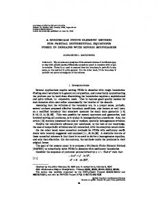
FIG. 10. 共Color online兲共a兲Woven nanostructure of carbon nanotubes; 共b兲 the woven nanostructure subject to a point force of 50 eV/ nm as indicated; 共c兲 the structure with a broken carbon nanotube away from the point force of 50 eV/ nm; 共d兲 the structure with a broken carbon nanotube underneath the point force of 50 eV/ nm. The contours are used to distinguish displacements of atoms as shown with blue representing the neutral position and the red maximal deflection. 035435-6


ATOMIC-SCALE FINITE ELEMENT METHOD IN… VI. APPLICATION OF AFEM TO WOVEN NANOSTRUCTURE OF CARBON NANOTUBES

Some complex atomic structures involving a large number of atoms with multiple kinds of atomistic interactions can be efficiently studied by AFEM on simple computational platforms such as personal computers.16 For example, structured composites possess designed mechanical, thermal, and electrical properties, and are provided in many forms in synthetic materials and exist in many biological systems in nature. The woven structure of CNT fibers has already been realized.25 The woven nanostructure of individual CNTs, as shown in Fig. 10共a兲, is another representative candidate for exploiting the superior mechanical properties of CNT. It has the potential for unique applications, where ultimate toughness, strength and lightness are required, such as in body armor and aerospace product. Such a nanostructure is still difficult to assemble with the existing experimental technique, and is also a challenge for atomistic studies. Here we use AFEM to study this woven nanostructure of CNTs. Figure 10共a兲 shows ten 共5,5兲 CNTs with 16 000 atoms that form a woven nanostructure with an intertube spacing of 3.86 nm. The interactions within the same CNT are characterized by Brenner’s potential13 with the AFEM element in Fig. 1. Between CNTs, atoms interact through the van der Waals potential for carbon,26 and nonlinear string elements incorporating such potential are used. The centers of end cross sections of all CNTs are on the same horizontal plane. Each end cross section has two atoms in the horizontal plane, and these atoms are fixed. The atomic structure shown in Fig. 10共a兲 corresponds to the relaxed, equilibrium state. Figure 10共b兲 shows the deformed atomic structure subject to a vertical point force of 50 eV/ nm at the center. The contours in Fig. 10共b兲 represent different levels of the displacements of atoms, where displacements are measured from the relaxed, equilibrium configuration in Fig. 10共a兲. The deflection, which is the displacement at the bottom of woven nanostructure 共below the loading point兲, is 1.70 nm, while for comparison, the deflection in a single CNT subject to the same force 共Fig. 4兲 is 3.08 nm, i.e., more than 80% larger. For the same structure subject to a lateral force of 50 eV/ nm in the horizontal plane, the resulting displacement is 2.38 nm. Therefore, the woven nanostructure is much stiffer than a single CNT since all CNTs contribute to the stiffness. We further examine the sensitivity of woven nanostructure to defects. Figure 10共c兲 shows the deformed atomic

1

F. F. Abraham, R. Walkup, H. Gao, M. Duchaineau, T. Diaz De La Rubia, and M. Seager, Proc. Natl. Acad. Sci. U.S.A. 99, 5777 共2002兲. 2 F. F. Abraham, R. Walkup, H. Gao, M. Duchaineau, T. Diaz De La Rubia, and M. Seager, Proc. Natl. Acad. Sci. U.S.A. 99, 5783 共2002兲. 3 G. E. Moore, Electronics 38, 114, 共1965兲. 4 Stable atomic structure means no significant amount of atom bond breaking or formation of new bonds, while well-defined

structure, with one neighbor CNT broken. The structure is subject to the same vertical force of 50 eV/ nm. The deflection is 2.01 nm, slightly larger than 1.70 nm for a perfect structure. In another case, where the top CNT underneath the force is broken, as shown in Fig. 10共d兲, the deflection is only 1.58 nm, which is even smaller than 1.70 nm for a perfect structure. This is because breaking of top CNT causes upward springback of the bottom CNT. This suggests that the woven nanostructure is insensitive to structural defects. If the woven structure involves more CNTs, it should have even higher stiffness and be less sensitive to defects. VII. CONCLUDING REMARKS AND DISCUSSION

We have developed an atomic-scale finite element method 共AFEM兲 which has exactly the same formal structure as continuum FEM, and therefore can be seamlessly combined with continuum FEM in multiscale computation. AFEM uses both first and second order derivatives of system energy, and is faster than the standard conjugate gradient method. For stable atomic structures and well-defined interatomic potentials, AFEM possesses order-N characteristics and is suitable for large scale problems, particularly after being combined with continuum FEM. AFEM is applicable to many atomistic studies since it can incorporate other atomistic models such as tight-binding potential. Through continuous update of AFEM elements according to current positions of atoms, AFEM can also model the evolution of atomic structure. In fact, the string elements for van der Waals interaction are updated in the study of the woven nanostructure of CNTs in Fig. 10. We have already demonstrated that some rather complex problems can be studied via AFEM on a personal computer. Together with parallel computation technique, the combined AFEM/FEM is most effective for treating problems with a large number of degrees of freedom, and therefore significantly increases the speed as well as the system size in large scale computation. Many optimization problems involving a large number of variables can also be efficiently solved with AFEM if the corresponding K 共matrix of second-order derivatives兲 is sparse. ACKNOWLEDGMENTS

This research was supported by NSF 共Grant Nos. 0099909, 01-03257, and 0328162兲, Office of Naval Research 共Grant No. N00014-01-1-0205, Program Officer Dr. Y.D.S. Rajapakse兲, and NSFC.

interatomic potential refers to no drastic oscillatory behavior. These ensure that energy surface has no drastic changes and is smooth. 5 R. E. Rudd and J. Q. Broughton, Phys. Status Solidi B 217, 251 共2000兲. 6 V. B. Shenoy, R. Miller, E. b. Tadmor, D. Rodney, R. Phillips, and M. Ortiz, J. Mech. Phys. Solids 47, 611 共1999兲. 7 S. Curtarolo and G. Ceder, Phys. Rev. Lett. 88, 255504 共2002兲. 8 W. E. and Z. Huang, Phys. Rev. Lett. 87, 135501 共2001兲.

035435-7


LIU et al. 9 H.

Rafii-Tabar, L. Hua, and M. Cross, J. Phys.: Condens. Matter 10, 2375 共1998兲. 10 S. Kohlhoff, P. Gumbsch, and H. F. Fischmeister, Philos. Mag. A 64, 851 共1991兲. 11 W. Yang, H. Tan, and T. F. Guo, Modell. Simul. Mater. Sci. Eng. 2, 767 共1994兲. 12 J. Tersoff, Phys. Rev. Lett. 61, 2879 共1988兲. 13 D. W. Brenner, Phys. Rev. B 42, 9458 共1990兲. 14 D. W. Brenner, O. A. Shenderova, J. A. Harrison, S. J. Stuart, B. Ni, and S. B. Sinnott, J. Phys.: Condens. Matter 14, 783 共2002兲. 15 W. H. Press, S. A. Teukolsky, W. T. Vetterling, and B. P. Flannery, Numerical Recipes 共Cambridge University Press, New York, 1986兲. 16 All computations are performed on a PC with 2.8 GHz CPU and 1 G memory. 17 Corresponding CPU time is 24 min, which is about 50% longer than the linear projection from Fig. 4. This increase in CPU time is due to the reduced speed of data access in a PC for large problems. 18 IMSL, IMSL共R兲 Fortran 90 MP Library Version 4.01, McGraw-Hill,

San Ramon, 1999. B. I. Yakoboson, C. J. Brabed, and J. Bernholc, Phys. Rev. Lett. 76, 2511 共1996兲. 20 ABAQUS, Inc. is the world’s leading provider of software for advanced finite element analysis. The headquarter is located at 166 Valley St., Providence, RI 02909-2499. 21 T. W. Tombler, C. Zhou, L. Alexseyev, J. Kong, H. Dai, L. Liu, C. S. Jayanthi, M. Tang, and S. Wu, Nature 共London兲 405, 769 共2000兲. 22 P. Zhang, Y. Huang, P. H. Geubelle, P. A. Klein, and K. C. Hwang, Int. J. Solids Struct. 39, 3893 共2002兲. 23 B. Chen, Y. Huang, H. Gao, and W. Yang, Int. J. Solids Struct. 41, 1 共2004兲. 24 B. Chen, Y. Huang, H. Gao, and P. D. Wu, Int. J. Solids Struct. 41, 2293 共2004兲. 25 A. B. Dalton, S. Collins, E. Munoz, J. M. Razal, V. H. Ebron, J. P. Ferraris, J. N. Coleman, B. G. Kim, and R. H. Baughman, Nature 共London兲 423, 703 共2003兲. 26 L. A. Girifalco, M. Hodak, and R. S. Lee, Phys. Rev. B 62, 13104 共2000兲. 19

035435-8