Computer Modeling in Engineering and Sciences, vol.26, no.2, pp.91-106, 2008
Atomic-scale modeling of self-positioning nanostructures Y. Nishidate1 and G. P. Nikishkov1,2
Abstract: Atomic-scale finite element procedure for modeling of self-positioning nanostructures is developed. Our variant of the atomic-scale finite element method is based on a meshless approach and on the Tersoff interatomic potential function. The developed algorithm is used for determination of equilibrium configuration of atoms after nanostructure self-positioning. Dependency of the curvature radius of nanostructures on their thickness is investigated. It is found that for thin nanostructures the curvature radius is considerably smaller than predicted by continuum mechanics equations. Curvature radius variation with varying orientation of crystallographic axes is also modeled and results are compared to finite element continuum anisotropic solution. keyword: Nanostructure, Self-positioning, Atomicscale finite element method. 1 Introduction Nanoscale structures have many potential applications. However, controlling and manipulating formation of nanoscale structures is usually complicated. One promising approach to creation of 3D nanoscale structures is the method utilizing self-positioning phenomena of thin solid films [Schmidt and Eberl (2001); Songmuang, Deneke, and Schmidt (2006); Golod, Prinz, Mashanov, and Gutakovsky (2001); Vaccaro, Kubota, and Aida (2001)]. The self-positioning is caused by lattice mismatching strain in layered structures composed of several metal or semiconductor materials. The self-positioning structures are created by depositing a sacrificial material layer and several lattice mismatched layers. After etching away the sacrificial layer, the layered materials form hinges or tubes with diameter controllable by layer material properties and thickness. Strain-driven self-positioning can be used to create 3D nanoscale structures by folding 2D membranes as origami (Japanese pa1 University
of Aizu, Aizu-Wakamatsu 965-8580, Japan author, email:
[email protected]
2 Corresponding
per craft work) [In, Kumar, Shao-Horn, and Barbastathis (2006); Arora, Nichol, Smith, and Barbastathis (2006)]. This approach is simple and robust, and deformation is predictable and controllable. Analytical continuum mechanics approaches [Hsueh (2002); Nikishkov (2003); Nishidate and Nikishkov (2006)] and computational finite element modeling [Nikishkov, Khmyrova, and Ryzhii (2003); Nikishkov, Nishidate, Ohnishi, and Vaccaro (2006)] have been applied to estimating deformations of self-positioning multilayer structures. However, these approaches do not take into account atomic-scale effects like absence of neighboring atoms at free surfaces. Recently, atomic-scale modeling has been applied to practical systems consisting of hundreds of thousands of atoms[Fitzgerald, Goldbeck-Wood, Kung, Petersen, Subramanian, and Wescott (2008)]. Several finite element algorithms have been developed for multiscale simulations [Theodosiou and Saravanos (2007); Chirputkar and Qian (2008)]. The atomic-scale finite element method (AFEM) based on the Brenner interatomic potential has been proposed for multi-scale analysis of carbon nanotubes [Liu, Huang, Jiang, Qu, and Hwang (2004); Liu, Jiang, Huang, Qu, Yu, and Hwang (2005)]. We have applied the AFEM to modeling of self-positioning bilayer structures. The investigation of curvature radius dependence on the structure thickness [Nishidate and Nikishkov (2007)] showed that atomic-scale and continuum mechanics solutions produce same results for structures with thickness larger than 100 nm. Atomic scale effects play significant role for thin self-positioning nanostructures. In this article, formulation of the atomic-scale finite element method with the use of of the Tersoff-Nordlund potential function is presented. Since the self-positioning of nanostructures involves large translations and rotations, a special iteration procedure that includes load relaxation factor is developed. The created AFEM code is applied to modeling of bi-layer self-positioning nanostructures. Deformation of self-positioning structures with
92
Computer Modeling in Engineering and Sciences, vol.26, no.2, pp.91-106, 2008
varying thickness and with varying orientations of crys- bonds without external loads, total energy E is replaced by a potential energy. Expressions of energy derivatives tallographic axes is investigated. should be obtained to formulate the AFEM global equation system, so energy function E should be at least twice 2 Atomic-scale finite element method differentiable. The atomic-scale finite element method (AFEM) is proEquation (1) shows that solution becomes less reliable posed for analysis of carbon nanotubes [Liu, Huang, as current configuration gets further from equilibrium Jiang, Qu, and Hwang (2004); Liu, Jiang, Huang, Qu, atomic configuration. Self-positioning structures deform Yu, and Hwang (2005)]. The atomic-scale finite element with large trandslational and rotational displacements, so equation system is derived from the approximation of enit is desirable to divide loading into several steps and to ergy E around current configuration x(i) : apply load gradually. Therefore, we employ the following Newton-Raphson iteration procedure to obtain the fi∂E |x=x(i) ·(x − x(i) ) E(x) ≈ E(x(i) ) + nal structure shape. ∂x ∂2 E 1 + (x − x(i) )T · 2 |x=x(i) ·(x − x(i) ), (1) do 2 ∂x K = K(x(i) ) f = f(x(i) ) and its subsequent minimization: α = g(K, f) ∂E f = α f(x(i) ) = 0. (2) (6) ∂x ∆u = K−1 f x(i+1) = x(i) + ∆u Substituting equation (1) into (2), AFEM global equation u(i+1) = u(i) + |∆u| system can be obtained, and expressed in a form similar |∆u| to conventional finite element equation system: while (i+1) > ε u Ku = f, (3) At each updated configuration, tangent stiffness matrix where K is a global stiffness matrix, u is a displacement and loading vector should be calculated using equation vector, and f is a load (force) vector. In the AFEM, the (4) and (5). In the iteration procedure, ε is an error tolglobal stiffness matrix K and the load vector f are com- erance, g is a function for estimating load relaxation facposed of second and first derivatives of the system energy tor α. Constant α factor throughout overall solution can perform unnecessary iterations or can lead to divergence, with respect to atom positions: because derivative (slope) of the interaction potential enµ 2 ¶ µ 2 ¶ ergy usually becomes smaller as current configuration ∂ E ∂ E ··· ∂x1 ∂x1 gets closer to equilibrium where loading becomes zero. ∂x1 ∂xn 3×3 3×3 . . . . .. . (4) The relaxation factor is estimated at each loading step K= , µ 2 . ¶ µ 2 . ¶ using tangent stiffness matrix and current loading vector. ∂ E ∂ E ··· In our case, the value of α is calculated as: ∂xn ∂x1 3×3 ∂xn ∂xn 3×3 umean ¶ µ , u= ∂E a n ¯µ i ¶¯ − 1 ¯¯ f1 f2i f3i ¯¯ ∂x 1 1×3 umean = ∑ ¯ ¯, ii , K ii , K ii .. n i=0 K11 (7) 22 33 , (5) f= . ¶ µ 1, u ≤ δ, ∂E α= δ − ∂xn 1×3 , u > δ, u where E is the total energy of the atomic system, n is a number of atoms (AFEM nodes), and xi is the coor- where n is a number of atoms, f ji is a j-th component of dinate vector of an i-th atom. As long as the problem full load vector acting on i-th atom, K iijj are correspondis to find the static equilibrium configuration of atomic ing diagonal entries of current tangent stiffness matrix,
Atomic-scale modeling of self-positioning nanostructures
93
Figure 1 : Self-positioning GaAs-InAs bi-layer hinge before and after self-positioning. a is a characteristic length of atomic system, and δ is a displacement suppression factor representing admissible mean displacement length. We selected characteristic length a as an initial lattice period, and a constant δ with the value 2 · 10−4 . Stronger load relaxation is applied if smaller δ is selected, or calculated mean value of the solution guess umean increases. 3 Modeling GaAs and InAs crystalline structures We model bi-layer self-positioning hinges consisting of GaAs top and InAs lower layer (Fig. 1). Coordinate axes x, y, and z are aligned to structure length, thickness, and width (bending axis) directions, respectively. Figure 2 : Atomic configuration and bonding in An AFEM mesh is constructed in accordance with GaAs zincblende crystalline structures. There are eight corner and InAs crystalline structures called zincblende crystal. and six face center atoms (bigger) and four inner atoms Arrangement of atoms in zincblende crystals is shown in (smaller). Fig. 2. Arsenide atoms occupy crystal corners and face centers of the unit crystal, and Gallium/Indium atoms are inside with positions (0.25, 0.25, 0.25), (0.75, 0.25, 0.75), (0.25, 0.75, 0.75), and (0.75, 0.75, 0.25) in the unit scribes interatomic interactions. Several empirical interedge length crystal. The GaAs and InAs possess material anisotropy depend- atomic potential functions have been developed to study ing on its crystal orientation. We investigate the effect behavior of atomic systems [Brenner (1990); Brenner, of anisotropy depending on a material orientation an- Shenderova, Harrison, Stuart, Ni, and Sinnott (2002); gle. The material orientation angle is modeled by ro- Tersoff (1989)]. For example, Liu, Huang, Jiang, Qu, and tating crystals around global y axis. Fig. 3 shows the Hwang (2004); Liu, Jiang, Huang, Qu, Yu, and Hwang procedure of creation AFEM meshes for modeling GaAs (2005) employed an empirical interatomic potential funcand InAs material anisotropy. The original crystalline tion and its parameters developed by Brenner (1990); structure with zero material orientation angle is prepared. Brenner, Shenderova, Harrison, Stuart, Ni, and Sinnott Then the structure is rotated around y axis and atoms out- (2002).
Although the Brenner potential model is widely used and successfully applied for modeling several types of atomic structures, its parameters for Indium, Gallium, 4 Modeling In–Ga–As atomic interaction and Arsenide systems are not available. Another empiriThe atomic-scale finite element method employs contin- cal potential energy model has been proposed by Tersoff uous empirical interatomic potential function which de- (1989). In the Tersoff model, total potential energy E is side the rectangular solution domain are removed.
94
Computer Modeling in Engineering and Sciences, vol.26, no.2, pp.91-106, 2008
l x
Unit crystal
z
x
x
w
z
z
(a)
(b)
(c)
Figure 3 : Modeling atomic structures with different material axes orientation. (a) Initial structure with unit crystals aligned to global axes. (b) Structure rotation around y axis by specified orientation angle. (c) Removal of atoms outside a rectangular region. Appearance of the potential function (8) is slightly different from the original Tersoff potential function due to subsequent parametrization by Nordlund, Nord, Frantz, and Keinonen (2000) for Indium, Gallium and Arsenide systems. The parameter values for Indium, Gallium, and Arsenide systems are listed in Tab. 1.
given by the following function: E = ∑ Ei = i
1 ∑ Vi j , 2∑ i j6=i
Vi j = fC (ri j ) [ fR (ri j ) + bi j fA (ri j )] , fR (ri j ) = Ai j exp(−λi j ri j ), fA (ri j ) = −Bi j exp(−µi j ri j ), ri j ≤ Ri j , 1, h i ri j −Ri j 1 1 fC (ri j ) = 2 + 2 cos Si j −Ri j π , Ri j < ri j < Si j , 0, Si j ≤ ri j , n
n
bi j = (1 + βi ji j ζi ji j )−1/(2ni j ) , ζi j =
∑
fC (rik )g(θi jk ),
The parameters obtained by Nordlund correspond to basic elastic and melting crystal properties. They were developed for investigation of damage at Si/Ge, AlAs/GaAs, and InAs/GaAs interfaces. It was noted that the parameters should be used with care for other pur(8) poses. So, we performed several tests to confirm parameter suitability for our modeling of self-positioning structures. The first test measured correspondence of elastic properties obtained using the Nordlund parameters to elastic properties known from the literature. The second test involved calculation of lattice parameters for GaAs and InAs and their comparison to known values.
k6=i, j
g(θi jk ) = 1 +
c2ik c2ik − , dik2 dik2 + (hik − cosθi jk )2
where Ei is the potential energy of atom i, Vi j the potential energy of a bond i– j, ri j the distance from atom i to atom j, fC the cut-off function to disregard effects from distant atoms, fR a reactive component, fA an attractive component, and bi j a bonding term to represent multi-atom interaction effects characterized by bonding angles.
Using the AFEM with Tersoff potential and Nordlund parameters, elastic properties of GaAs and InAs are estimated by applying external load at the end of specimen shaped into a thin rod along its longitudinal direction. Strain and stress are calculated at a position sufficiently far from the free end where external load is applied. Taking into account that the specimen is thin in transverse directions, Young’s modulus E and Poisson’s ratio ν are determined by: E=
σx , εx
ν=−
εy . εx
(9)
95
Atomic-scale modeling of self-positioning nanostructures
Table 1 : Tersoff potential energy parameters for Indium, Gallium, and Arsenide systems fit by Nordlund, Nord, Frantz, and Keinonen (2000) In–Ga In–In In–As As–As Ga–As Ga–Ga n 3.43739 3.40223 0.7561694 0.60879133 6.31741 3.4729041 c 0.0801587 0.084215 5.172421 5.273131 1.226302 0.07629773 d 19.5277 19.2626 1.665967 0.75102662 0.790396 19.796474 h 7.26805 7.39228 −0.5413316 0.15292354 −0.518489 7.1459174 β 0.705241 2.10871 0.3186402 0.00748809 0.357192 0.23586237 −1 ˚ ) λ (A 2.5616 2.6159 2.597556 2.384132239 2.82809263 2.50842747 −1 ˚ ) µ (A 1.58314 1.68117 1.422429 1.7287263 1.72301158 1.490824 A (eV ) 1719.7 2975.54 1968.295443 1571.86084 2543.29720 993.888094 B (eV ) 221.557 360.61 266.571631 546.4316579 314.459660 136.123032 ˚ R (A) 3.4 3.5 3.5 3.4 3.4 3.4 ˚ S (A) 3.6 3.7 3.7 3.6 3.6 3.6
For a cubic crystal with axes aligned with cube edges, estimation of Young’s modulus and Poisson’s ratio from constitutive tensor components C11 and C12 can be made as follows: E=
(C11 −C12 )(C11 + 2C12 ) , C11 +C12
the problem size parameters c = 1, 2, 4, 8, 12, 16, 24, and 36 prepared to find equilibrium configuration. We model material anisotropy with material orientation angles 0, 15, 30, 45, 60, 75, and 90 degrees. Appearance of crystalline structure geometry is shown in Fig. 5 for C12 ν= . (10) varying orientation angles. C11 +C12
The lattice period is estimated at the center of cube structures consisting of several crystals in all directions. Elastic properties and lattice periods estimated by the AFEM modeling for GaAs and InAs are compared with experimental values [Bhattacharya (1993)] in Tab. 2. A difference of 5% is observed for Young’s modulus of GaAs, however in general the correspondence of estimated elastic properties to their experimental values is acceptable. Estimated lattice periods are in very good agreement with experimental values. We therefore concluded that the AFEM with Tersoff potential and parameters developed by Nordlund is suitable for simulation of the atomic-scale behaviour of nanostructures composed of GaAs and InAs.
y (thickness)
x (length) t2 t1 z (width)
GaAs 3a 0 c InAs 1a 0 c 16 a 0 c
Figure 4 : Schematic of a self-positioning problem. The number of atoms in the problem is determined by the parameter c.
The top GaAs and lower InAs layer are composed of 3c and c number of crystals in the thickness (y) direc5 Modeling self-positioning GaAs–InAs hinges tion. In the length (x) direction, several atomic layers of A self-positioning structure consisting of GaAs top and length 16a0 c is prepared where a0 is an initial lattice peInAs lower layers is shown in Fig. 4. It is used for investi- riod (Fig. 4). For hinge with 0 orientation angle, 16a0 c is gation of curvature radius dependence on structure thick- equals to length of 16 unit crystals. ness and crystal orientation angle. We employ problem We compare results obtained by AFEM with analytical size parameter c to express size of atomic systems. Cur- continuum mechanics solution under plane strain condivature radius of GaAs and InAs bilayer structures with tions [Nikishkov (2003)]. The plane strain conditions
96
Computer Modeling in Engineering and Sciences, vol.26, no.2, pp.91-106, 2008
Table 2 : GaAs and InAs properties: comparison of AFEM estimation with literature [Bhattacharya (1993)].
E (GPa) ν LP (nm)
Experiment 85.3 0.312 0.56533
GaAs AFEM 81.0 0.313 0.56389
δ (%) −5.04 0.32 −0.25
Experiment 51.8 0.352 0.60584
InAs AFEM 51.4 0.357 0.60592
δ (%) −0.77 1.42 0.01
correspond to structures with infinite width in z direction. In order to simulate atomic systems of infinite dimensions, periodic boundary conditions, which help to minimize number of atoms in the model are usually employed in computational modeling.
done with care when calculating curvature radius using an analytical technique. It is appropriate to add some offset equal to a ’radius’ of an atom at each free surface. While adding such an offset is not critical for thick structures, it can be important for problems with small number Periodic boundary conditions in the z (width) direction of crystals in y direction. are applied for structures with orientation angles 0, 45 If we adopt half of the atom connectivity length as an and 90 degrees. Such structures consist of one complete offset, then √ for zincblende crystal structures the offset is and another incomplete crystal in the width direction, equal to 3a/8, where a is a lattice period. Correspondand connection across periodic boundary is created when ing offsets are 0.1224 nm for GaAs and 0.1425 nm for InAs. looking for neighboring atoms. For hinges with the other orientation angles (15, 30, 60 Initial strains ε0i in equation (11) are determined by initial and 75 degrees), enough number of atomic layers corre- (a0 ) and material-specific lattice period (ai ) as: sponding to width 30a0 are prepared and displacement is ai − a0 0 . (12) constrained in the width direction to imitate plane strain εi = a0 conditions (εz = 0). Boundary condition restricting displacements in x direc- We determine the initial lattice period for the bi-layer system using a weighted linear interpolation of GaAs and tion at one end of the structure are also applied. InAs specific lattice periods: The analytical continuum mechanics solution is used for comparison. In addition, in order to to reduce computing a = a1 n1 + a2 n2 , (13) 0 n1 + n2 time, the initial configuration of atoms in AFEM meshes is determined according to the curvature radius given by where n1 and n2 are number of crystals in each InAs and continuum mechanics solution under plane strain condi- GaAs layer. Therefore, a0 is assumed to be 0.57546 nm tions [Nikishkov (2003)]: in our problems. E10 2t14 + E20 2t24 + 2E10 E20 t1t2 (2t12 + 2t22 + 3t1t2 ) , R= 6E10 E20 t1t2 (t1 + t2 )(η1 ε01 − η2 ε02 ) Ei , ηi = 1 + νi , Ei0 = 1 − ν2i
(11)
6 Numerical results The developed AFEM computer program was used to solve two problem series for self-positioning nanostructures. The first one is computing the curvature radius of bi-layer hinges with varying thickness. The second series includes problems with varying orientation of material axes for the same nanostructures.
where Ei , νi , ti , and ε0i are Young’s modulus, Poisson’s ratio, thickness, and initial lattice mismatching strain, respectively. Subscripts 1 and 2 denote material layers. In bi-layer systems, expression is symmetric to each other, so distinction of layer 1 and 2 for curvature radius calcu6.1 Curvature dependence on the structure thickness lation is not important.
Definition of thickness for structures consisting of just Bi-layer atomic structures of different thickness are crea few crystal layers in the thickness direction should be ated by setting problem size parameter c to 1, 2, 4, 8,
Atomic-scale modeling of self-positioning nanostructures
0◦
97
15◦
Figure 6 : Final shape of atomic bi-layer structure with the size c = 1. 30◦
45◦ are used to calculate curvature radius at the neutral layer by linear interpolation. The neutral layer is located at 0.54 of the thickness from the bottom of the structure in our problems.
Fig. 6 shows the final shape of an atomic model after selfpositioning in case of problem size c = 1, totally four unit crystals in the thickness direction. Analysis reveals that spacing of atoms is smaller in GaAs and larger in InAs, and that the free end is not straight along local thickness 60◦ 75◦ direction, due to expansion in the lower layer and comFigure 5 : Top view of atom configurations for self- pression in the top layer. positioning hinges with different orientation angles. Ori- In order to estimate convergence of the curvature radius entation angles 0, 45, and 90 degrees have periodic with thickness increase, least square fits of the obtained boundary in z (width) direction. eight numerical solutions are performed using power
12, 16, 24, and 36. Corresponding thicknesses are 2.56, 4.86, 9.46, 18.65, 27.84, 37.03, 55.41 and 82.98 nm. The equilibrium configurations of bi-layer hinges are determined with the use of Newton-Raphson iteration procedure (6). We compare the AFEM values of curvature radius with the continuum mechanics solution under plane strain conditions [Nikishkov (2003)]. In the continuum mechanics solution, elastic properties estimated by the AFEM on the tensile rod model are used (see Tab. 2). Curvature radius values based on the AFEM modeling at the top and at the bottom of the atomic structures are calculated by taking three neighbor nodes along the x direction to fit a circle at each y level. Then, these values
function R(c) = α1 (α2 c + α3 )−β + γ, where c indicates size of the atomic system, and α1 , α2 , α3 , β, and γ are parameters found by least square fit, where γ corresponds to converged value for infinite number of crystal layers. Fig. 7 shows the ratio of the curvature radius determined by the AFEM and the continuum mechanics solution with varying thickness. Least square fits indicate that the relative difference of curvature radius converges to 1.0037 for an infinite number of atomic layers. For the biggest problem we investigated (c = 36), the difference is −0.36%. So, the AFEM and continuum mechanics solution are in quite good agreement for large thickness. The difference between atomic-scale and continuum mechanics curvature radius increases with reduction of the structure thickness.
Computer Modeling in Engineering and Sciences, vol.26, no.2, pp.91-106, 2008
1.05
1.4
1.00
1.3 RAFEM/RCont.
RAFEM/RCont.
98
0.95 0.90 0.85
1.2 1.1 1.0
c=8 c=4 c=2
0.9
0.80 0
20
40 60 80 Thickness (nm)
100
120
0.8 0
15
30 45 60 Orientation angle (degrees)
75
c=1 90
Figure 7 : Ratio of the curvature radius determined by Figure 9 : Dependency of RAFEM /RCont.(0◦ ) on orientathe AFEM and the continuum mechanics solution with tion angle for problem sizes c = 1 to 8. varying thickness. 7 Conclusion This difference is −18.4% for c = 1, corresponding to Algorithm of the atomic-scale finite element method four unit crystals in the thickness direction and thickness based on the Tersoff interatomic potential has been de2.56 nm. veloped. Solution procedure for problems with large displacements is organized as the Newton-Raphson iteration 6.2 Curvature dependence on the material orientation procedure. A load relaxation factor is introduced in order angle to restrict load step magnitude for cases with high gradients of the atomic system energy. AFEM solutions with problem sizes c = 1, 2, 4 and 8 and material orientation angles 0, 15, 30, 45, 60, 75 and 90 de- The developed AFEM code is applied to modeling of grees are performed for modeling anisotropy of GaAs GaAs and InAs bi-layer self-positioning nanostructures. and InAs bi-layer nanostructures. Fig. 8 shows the final Two problem series include investigation nanohinge curshape of atomic models after self-positioning in case of vature radius dependence on the structure thickness and crystal size c = 1 for orientation angles 0, 15, 30, 45, 60 the material orientation angle. The self-positioning hinge deformation converges to the continuum mechanics soluand 75 degrees. tion under plane strain conditions with increasing strucTab. 3 contains ratios of the curvature radius R to the ture thickness. However, for nanostructures of small thickness t obtained by the AFEM modeling at the neuthickness less than 40 nm atomic-scale effects play contral layer for orientation angles 0, 15, 30 and 45 degrees siderable role. Dependency of curvature radius on the and by continuum mechanics solution for zero orientamaterial orientation angle shows periodic curve with the tion angle. For varying orientation angles, the ratio in maximum curvature radius observed for orientation anbetween maximum and minimum values of curvature ragle 45 degrees. Our modeling shows that hinges with dius is about 1.35. This ratio is similar to experimendifferent material orientation angles can exhibit curvatal data and numerical finite element modeling of GaAs ture radius differing by 35%. and In0.2 Ga0.8 As bi-layer structures [Nikishkov, Nishidate, Ohnishi, and Vaccaro (2006)] References Fig. 9 shows dependency of the curvature radius ratio (RAFEM /RCont.(0◦ ) ) for varying material orientation angle. Arora, W. J.; Nichol, A. J.; Smith, H. I.; BarbasCurvature radius is the minimum at orientation angles 0 tathis, G. (2006): Membrane folding to achieve threeand 90 degrees and maximum at 45 degrees, and depen- dimensional nanostructures: Nanopatterned silicon nidency on orientation angle shows a curve similar to sinu- tride folded with stressed chromium hinges. Appl. Phys. soidal function with frequency π. Lett., vol. 88, pp. 053108–1–3.
99
Atomic-scale modeling of self-positioning nanostructures
0◦
15◦
30◦
45◦
60◦
75◦
Figure 8 : Final shape of atomic bi-layer structure with the size c = 1 for orientation angles 0 to 75 degrees. Bhattacharya, P. (1993): Properties of Lattice- Chirputkar, S. U.; Qian, D. (2008): Coupled AtomMatched and Strained Indium Gallium Arsenide. Insti- istic/Continuum Simulation based on Extended SpaceTime Finite Element Method. CMES: Computer Modtution of Electrical Engineers, London. Chap. 1.2. eling in Engineering & Sciences, vol. 24, no. 3, pp. 185– Brenner, D. W. (1990): Empirical potential for hy- 202. drocarbons for use in simulating the chemical vapor deposition of diamond films. Phys. Rev. B, vol. 42, pp. Fitzgerald, G.; Goldbeck-Wood, G.; Kung, P.; Petersen, M.; Subramanian, L.; Wescott, J. (2008): 9458–9471. Materials Modeling from Quantum Mechanics to The Brenner, D. W.; Shenderova, O. A.; Harrison, J. A.; Mesoscale. CMES: Computer Modeling in Engineering Stuart, S. J.; Ni, B.; Sinnott, S. B. (2002): A second- & Sciences, vol. 24, no. 3, pp. 169–183. generation reactive empirical bond order (REBO) potential energy expression for hydrocarbons. J. Phys.: Con- Golod, S. V.; Prinz, V. Y.; Mashanov, V. I.; Gutakovsky, A. K. (2001): Fabrication of conductdens. Matter, vol. 14, pp. 783–802.
100
Computer Modeling in Engineering and Sciences, vol.26, no.2, pp.91-106, 2008
Table 3 : Total thickness t (nm) and relative value of curvature radius R/t for problem sizes c = 1, 2, 4 and 8 with varying orientation angles. Dependency on orientation angle is symmetric in respect to orientation angle 45 degree. c 1 2 4 8
t (nm) 2.56 4.86 9.46 18.65
Cont. (0◦ ) 9.25 9.60 9.81 9.92
AFEM (0◦ ) 7.56 8.56 9.23 9.63
AFEM (15◦ ) 8.32 9.35 9.98 10.29
AFEM (30◦ ) 9.86 10.88 11.54 11.87
AFEM (45◦ ) 10.67 11.76 12.54 13.01
ing GeSi/Si micro- and nanotubes and helical microcoils. Nishidate, Y.; Nikishkov, G. P. (2006): Generalized plane strain deformation of multilayer structures with iniSemicond. Sci. Technol., vol. 16, pp. 181–185. tial strains. J. Appl. Phys., vol. 100, pp. 113518–1–4. Hsueh, C.-H. (2002): Modeling of elastic deformation of multilayers due to residual stresses and external bendNishidate, Y.; Nikishkov, G. P. (2007): Effect of thicking. J. Appl. Phys., vol. 91, no. 12, pp. 9652–9656. ness on the self-positioning of nanostructures. J. Appl. In, H. J.; Kumar, S.; Shao-Horn, Y.; Barbastathis, Phys., vol. 102, pp. 083501–1–5. G. (2006): Origami fabrication of nanostructured, three-dimensional devices: Electrochemical capacitors Nordlund, K.; Nord, J.; Frantz, J.; Keinonen, J. with carbon electrodes. Appl. Phys. Lett., vol. 88, pp. (2000): Strain-induced Kirkendall mixing at semicon083104–1–3. ductor interfaces. Comput. Mater. Sci., vol. 18, pp. 283– 294. Liu, B.; Huang, Y.; Jiang, H.; Qu, S.; Hwang, K. C. (2004): The atomic-scale finite element method. Comput. Methods Appl. Mech. Engrg., vol. 193, pp. 1849– Schmidt, O. G.; Eberl, K. (2001): Nanotechnology: Thin solid films roll up into nanotubes. Nature, vol. 410, 1864. pp. 168. Liu, B.; Jiang, H.; Huang, Y.; Qu, S.; Yu, M.-F.; Hwang, K. C. (2005): Atomic-scale finite element Songmuang, R.; Deneke, C.; Schmidt, O. G. (2006): method in multiscale computations with applications to Rolled-up micro- and nanotubes from single-material carbon nanotubes. Phys. Rev. B, vol. 72, pp. 035435–1– thin films. Appl. Phys. Lett., vol. 89, pp. 223109–1–3. 8. Nikishkov, G. P. (2003): Curvature estimation for mul- Tersoff, J. (1989): Modeling solid-state chemistry: Intilayer hinged structures with initial strains. J. Appl. teratomic potentials for multicomponent systems. Phys. Rev. B, vol. 39, pp. 5566–5568. Phys., vol. 94, no. 8, pp. 5333–5336. Nikishkov, G. P.; Khmyrova, I.; Ryzhii, V. (2003): Finite element analysis of self-positioning microstructures and nanostructures. Nanotechnology, vol. 14, pp. 820– 823.
Theodosiou, T. C.; Saravanos, D. A. (2007): Molecular Mechanics Based Finite Element For Carbon Nanotube Modeling. CMES: Computer Modeling in Engineering & Sciences, vol. 19, no. 2, pp. 121–134.
Nikishkov, G. P.; Nishidate, Y.; Ohnishi, T.; Vaccaro, P. O. (2006): Effect of material anisotropy on the self- Vaccaro, P. O.; Kubota, K.; Aida, T. (2001): Strainpositioning of nanostructures. Nanotechnology, vol. 17, driven self-positioning of micromachined structures. Appl. Phys. Lett., vol. 78, no. 19, pp. 2852–2854. pp. 1128–1133.
101
Atomic-scale modeling of self-positioning nanostructures
Appendix A:
First order differentiation of Tersoff potential for calculation of force vector
Tersoff potential function (8) is used to estimate forces acting on each atom. Assembly of first order derivatives of bonding i– j energy Vi j yields the global force vector. Let the distance ri j between atoms with positions xi and x j is defined as:
ri j = |ri j | = |x j − xi | Then derivatives of ri j in respect to atom positions xi and x j are:
x j − xi ∂ri j =− ∂xi ri j x j − xi ∂ri j = ∂x j ri j
Differentiation of Vi j in respect to positions xi , x j , and any neighboring atom position xk yields: · ½ ¾¸ ª ∂ri j ∂ fC © ∂Vi j ∂ fR ∂ fA = fR + bi j fA + fC + bi j ∂xi ∂xi ∂ri j ∂ri j ∂ri j ∂bi j + fC fA ∂xi · ½ ¾¸ ª © ∂ri j ∂ fC ∂Vi j ∂ fR ∂ fA = fR + bi j fA + fC + bi j ∂x j ∂x j ∂ri j ∂ri j ∂ri j ∂bi j + fC fA ∂x j ∂bi j ∂Vi j = fC fA ∂xk ∂xk Derivatives of bi j in respect to positions xi , x j , and xk have same appearance for all cases and is expressed as:
¢− 1 −1 ∂bi j ∂ζi j ¡ 1 = − βn ζn−1 1 + βn ζnij 2n ij ∂xi 2 ∂xi
∂cos(θi jk ) ∂g(θi jk ) ∂ζi j ∂rik ∂ fC = g(θi jk ) + fC ∂xi ∂xi ∂rik ∂xi ∂cos(θi jk ) ∂cos(θi jk ) ∂g(θi jk ) ∂ζi j = fC ∂x j ∂x j ∂cos(θi jk ) ∂cos(θi jk ) ∂g(θi jk ) ∂ζi j ∂rik ∂ fC = g(θi jk ) + fC ∂xk ∂xk ∂rik ∂xk ∂cos(θi jk ) Differentiation of cos(θi jk ) in respect to positions xi , x j , and xk :
∂cos(θi jk ) 1 = ∂xi (ri j rik )2 ¾¸ · ½ ∂ri j · rik ∂ri j ∂rik ri j rik − (ri j · rik ) rik + ri j ∂xi ∂xi ∂xi ¸ · ∂cos(θi jk ) ∂ri j ∂ri j · rik 1 = 2 ri j − (ri j · rik ) ∂x j ∂x j ∂x j ri j rik ¸ · ∂cos(θi jk ) ∂ri j · rik 1 ∂rik = rik − (ri j · rik ) 2 ∂xk ∂xk ∂xk ri j rik where ri j · rik denotes inner product of vectors ri j and rik . Differentiation of ri j · rik in respect to xi , x j , and xk :
© ª ∂ri j · rik = − (xk − xi ) + (x j − xi ) ∂xi ∂ri j · rik = (xk − xi ) ∂x j ∂ri j · rik = (x j − xi ) ∂xk Differentiation of g(θi jk ) in respect to cos(θi jk ): © ª 2c2 h − cos(θi jk ) ∂g(θi jk ) =h © ª2 i2 ∂cos(θi jk ) d 2 + h − cos(θi jk )
These are differentiations in respect to atom positions. In addition to these expressions, derivatives of fC , fA , fR in Differentiation of ζi j in respect to positions xi , x j , and respect to corresponding distances like ri j or rik should be given. xk :
102
Computer Modeling in Engineering and Sciences, vol.26, no.2, pp.91-106, 2008
Appendix B:
Second order differentiation of Tersoff potential for calculation of tangent stiffness matrix
The second order differentiation of Tersoff potential is calculated from first order differentiation. In second order differentiation, differentiation is calculated twice, so we employ superscript symbol to distinguish which is first or second differentiation symbol as following:
xm i
first differentiation symbol
xni
second differentiation symbol
∂2Vi j n = ∂xm i ∂xi
· ½ ¾¸ ª ∂2 ri j ∂ fC © ∂ fR ∂ fA f + b f + f + b + R ij A C ij n ∂xm ∂ri j ∂ri j i ∂xi ∂ri j " ∂ri j ∂ri j ∂2 fC ∂ fC ∂ fR ∂2 f R f + 2 + f + R C n ∂xm ∂ri j ∂ri j ∂ri2j ∂ri2j i ∂xi ( )# ∂2 fC ∂ fC ∂ fA ∂2 fA bi j fA + 2 + fC 2 + ∂ri j ∂ri j ∂ri2j ∂ri j ¶µ µ ¶ ∂ri j ∂bi j ∂bi j ∂ri j ∂ fC ∂ fA + f + f + A C n n ∂xm ∂xm ∂ri j ∂ri j i ∂xi i ∂xi fC fA
∂2 bi j n ∂xm i ∂xi
Second order differentiation of ri j in respect to atom positions xi and x j are:
(x j − xi )2 1 − ∂2 ri j ri j ri3j = m n (x j − xi )m (x j − xi )n ∂xi ∂xi − ri3j ∂2 ri j ∂2 ri j = m n= m n ∂xi ∂x j ∂x j ∂xi (x j − xi )2 1 −r + ri3j ij m (x j − xi ) (x j − xi )n ri3j
∂2Vi j = ∂xi ∂x j n xm i = xi n xm i 6= xi
n xm i = xj n xm i 6= x j
· ½ ¾¸ ª ∂2 ri j ∂ fC © ∂ fR ∂ fA fR + bi j fA + fC + bi j + ∂xi ∂x j ∂ri j ∂ri j ∂ri j " ∂ri j ∂ri j ∂2 fC ∂ fC ∂ fR ∂2 f R f + 2 + + f R C ∂xi ∂x j ∂ri2j ∂ri j ∂ri j ∂ri2j ( )# ∂2 fC ∂ fC ∂ fA ∂2 f A bi j fA + 2 + fC 2 + ∂ri j ∂ri j ∂ri2j ∂ri j ¶µ µ ¶ ∂ri j ∂bi j ∂bi j ∂ri j ∂ fC ∂ fA + fA + fC + ∂xi ∂x j ∂xi ∂x j ∂ri j ∂ri j fC fA
n For example, xm i equals to xi when first differentiation symbol is xi and second is xi , but not equal when first differentiation symbol is xi and second is yi .
Differentiation of Vi j in respect to positions xi , x j , and xk :
∂ri j ∂bi j ∂2Vi j = ∂xi ∂xk ∂xi ∂xk
µ
∂ fC ∂ fA fA + fC ∂ri j ∂ri j
∂2 bi j ∂xi ∂x j
¶ + fC fA
∂2 b i j ∂xi ∂xk
103
Atomic-scale modeling of self-positioning nanostructures
∂2Vi j = ∂x j ∂xi
Differentiation of bi j in respect to positions xi , x j , and xk has same appearance for all cases and expressed as:
· ½ ¾¸ ª ∂2 ri j ∂ fC © ∂ fR ∂ fA fR + bi j fA + fC + bi j + ∂x j ∂xi ∂ri j ∂ri j ∂ri j " ∂ri j ∂ri j ∂2 fC ∂ fC ∂ fR ∂2 f R f + 2 + f + R C ∂x j ∂xi ∂ri2j ∂ri j ∂ri j ∂ri2j ¢ 1 ∂2 bi j 1 n n−2 ¡ n n − 2n −2 ( )# = − β ζ 1 + β ζ i j ij n ∂xm 2 ∂2 fC ∂ fC ∂ fA ∂2 f A i ∂xi · bi j f + 2 + f + A C ¢ ∂ζi j ∂ζi j ¡ ∂ri j ∂ri j ∂ri2j ∂ri2j n n 1 + β ζ (n − 1) + i j m n ¶µ µ ¶ ∂x ∂x i i ∂ri j ∂bi j ∂bi j ∂ri j ∂ fC ∂ fA + fA + fC + ¢ ∂2 ζi j ¡ ∂xi ∂x j ∂xi ∂x j ∂ri j ∂ri j ζi j m n 1 + βn ζnij + ∂xi ∂xi ∂2 bi j ¶ ¸ µ fC fA 1 n ∂ζi j ∂ζi j n ∂x j ∂xi nβ − − 1 ζi j m n 2n ∂xi ∂xi
∂2Vi j = ∂xmj ∂xnj
· ½ ¾¸ Differentiation of ζi j in respect to positions xi , x j , and ª ∂2 ri j ∂ fC © ∂ fR ∂ fA + f f + b f + b + C R ij A ij xk : ∂xmj ∂xnj ∂ri j ∂ri j ∂ri j " ∂ri j ∂ri j ∂2 fC ∂ fC ∂ fR ∂2 f R f + 2 + + f R C ∂xmj ∂xnj ∂ri2j ∂ri j ∂ri j ∂ri2j ( )# ∂2 fC ∂ fC ∂ fA ∂2 fA ∂2 rik ∂ fC ∂rik ∂rik ∂2 fC bi j fA + 2 + fC 2 +∂2 ζi jk g(θi jk ) + = g(θ ) + ∂ri j ∂ri j ∂ri2j ∂ri j i jk n n n 2 ∂xm ∂xm ∂xm i ∂xi i ∂xi ∂rik i ∂xi ∂rik !µ à ¶ ∂ri j ∂bi j ∂bi j ∂ri j ∂ fC ∂ fA ∂rik ∂ fC ∂cos(θi jk ) ∂g(θi jk ) + m n fA + fC + + m n ∂x j ∂x j ∂x j ∂x j ∂ri j ∂ri j ∂xm ∂xni ∂cos(θi jk ) i ∂rik ∂rik ∂ fC ∂cos(θi jk ) ∂g(θi jk ) ∂2 bi j + fC fA m n ∂xni ∂rik ∂xm ∂cos(θi jk ) ∂x ∂x i j
∂ri j ∂bi j ∂2Vi j = ∂x j ∂xk ∂x j ∂xk
∂ri j ∂bi j ∂2Vi j = ∂xk ∂xi ∂xi ∂xk
∂2Vi j ∂xk ∂x j
=
∂ri j ∂bi j ∂x j ∂xk
µ
µ
∂ fC ∂ fA fA + fC ∂ri j ∂ri j
∂ fC ∂ fA fA + fC ∂ri j ∂ri j
µ
∂ fC ∂ fA fA + fC ∂ri j ∂ri j
j
fC
¶ + fC fA
∂2 bi j ∂x j ∂xk
+ fC fA
∂2 b i j ∂xk ∂xi
¶ + fC fA
∂2 b
ij
∂xk ∂x j
fC
∂cos(θi jk ) ∂cos(θi jk ) ∂2 g(θi jk ) ∂xm ∂xni ∂cos(θi jk )2 i
∂2 ζi jk ∂rik ∂ fC ∂cos(θi jk ) ∂g(θi jk ) = + ∂xi ∂x j ∂xi ∂rik ∂x j ∂cos(θi jk ) fC
∂2 bi j ∂2Vi j = fC fA ∂xk ∂xk ∂xk ∂xk
∂2 cos(θi jk ) ∂g(θi jk ) n ∂cos(θ ) + ∂xm i jk i ∂xi
∂2 cos(θi jk ) ∂g(θi jk ) + ∂xi ∂x j ∂cos(θi jk ) fC
∂cos(θi jk ) ∂cos(θi jk ) ∂2 g(θi jk ) ∂xi ∂x j ∂cos(θi jk )2
104
Computer Modeling in Engineering and Sciences, vol.26, no.2, pp.91-106, 2008
∂2 ζi jk ∂2 rik ∂ fC ∂rik ∂rik ∂2 fC g(θi jk ) + = g(θi jk ) + 2 ∂xi ∂xk ∂xi ∂xk ∂rik ∂xi ∂xk ∂rik ∂rik ∂ fC ∂cos(θi jk ) ∂g(θi jk ) + ∂xi ∂rik ∂xk ∂cos(θi jk ) ∂rik ∂ fC ∂cos(θi jk ) ∂g(θi jk ) + ∂xk ∂rik ∂xi ∂cos(θi jk ) fC
fC
∂2 cos(θi jk ) ∂g(θi jk ) + ∂xk ∂x j ∂cos(θi jk ) fC
∂cos(θi jk ) ∂cos(θi jk ) ∂2 g(θi jk ) ∂xi ∂xk ∂cos(θi jk )2
∂2 ζi jk ∂rik ∂ fC ∂cos(θi jk ) ∂g(θi jk ) = + ∂x j ∂xi ∂xi ∂rik ∂x j ∂cos(θi jk ) ∂2 cos(θi jk ) ∂g(θi jk ) + ∂x j ∂xi ∂cos(θi jk ) fC
∂cos(θi jk ) ∂cos(θi jk ) ∂2 g(θi jk ) ∂xi ∂x j ∂cos(θi jk )2
∂2 ζi jk ∂2 rik ∂ fC ∂rik ∂rik ∂2 fC = m n g(θi jk ) + m n 2 g(θi jk ) + m n ∂xk ∂xk ∂xk ∂xk ∂rik ∂xk ∂xk ∂rik ∂rik ∂ fC ∂cos(θi jk ) ∂g(θi jk ) + ∂xm ∂xnk ∂cos(θi jk ) k ∂rik ∂rik ∂ fC ∂cos(θi jk ) ∂g(θi jk ) + ∂xnk ∂rik ∂xm ∂cos(θi jk ) k fC
∂2 cos(θi jk ) ∂g(θi jk ) ∂2 ζi jk = fC + m n ∂x j ∂x j ∂xmj ∂xnj ∂cos(θi jk ) ∂cos(θi jk ) ∂cos(θi jk ) ∂2 g(θi jk ) ∂xmj ∂xnj ∂cos(θi jk )2
fC
∂2 ζi jk ∂rik ∂ fC ∂cos(θi jk ) ∂g(θi jk ) = + ∂x j ∂xk ∂xk ∂rik ∂x j ∂cos(θi jk ) fC
∂cos(θi jk ) ∂cos(θi jk ) ∂2 g(θi jk ) ∂xk ∂x j ∂cos(θi jk )2
∂2 cos(θi jk ) ∂g(θi jk ) + ∂xi ∂xk ∂cos(θi jk )
fC
fC
∂g(θi jk ) ∂2 ζi jk ∂rik ∂ fC ∂cos(θi jk ) = + ∂xk ∂x j ∂xk ∂rik ∂x j ∂cos(θi jk )
∂2 cos(θi jk ) ∂g(θi jk ) + n ∂xm k ∂xk ∂cos(θi jk )
fC
∂cos(θi jk ) ∂cos(θi jk ) ∂2 g(θi jk ) ∂xm ∂xnk ∂cos(θi jk )2 k
Differentiation of cos(θi jk ) in respect to positions xi , x j , and xk :
∂2 cos(θi jk ) ∂g(θi jk ) + ∂x j ∂xk ∂cos(θi jk ) fC
∂cos(θi jk ) ∂cos(θi jk ) ∂2 g(θi jk ) ∂x j ∂xk ∂cos(θi jk )2
∂2 ζi jk ∂2 rik ∂ fC ∂rik ∂rik ∂2 fC = g(θi jk ) + g(θi jk ) + 2 ∂xk ∂xi ∂xk ∂xi ∂rik ∂xk ∂xi ∂rik ∂rik ∂ fC ∂cos(θi jk ) ∂g(θi jk ) + ∂xk ∂rik ∂xi ∂cos(θi jk ) ∂rik ∂ fC ∂cos(θi jk ) ∂g(θi jk ) + ∂xi ∂rik ∂xk ∂cos(θi jk ) fC
∂2 cos(θi jk ) ∂g(θi jk ) + ∂xk ∂xi ∂cos(θi jk )
fC
∂cos(θi jk ) ∂cos(θi jk ) ∂2 g(θi jk ) ∂xk ∂xi ∂cos(θi jk )2
· ∂2 cos(θi jk ) 1 = 3 3 ri j rik n ∂xm ri j rik i ∂xi µ ¶ ½ 2 ∂ ri j · rik ∂ri j · rik ∂ri j ∂rik rik + ri j n n ri j rik + ∂xm ∂xm ∂xni ∂xi i ∂xi i µ ¶ ∂ri j · rik ∂ri j ∂rik rik + ri j m − (ri j · rik ) − n m ∂xi ∂xi ∂xi ¶¾ µ 2 ∂ri j ∂rik ∂ri j ∂rik ∂ ri j ∂2 rik n rik + ∂xm ∂xn + ∂xn ∂xm + ri j ∂xm ∂xn ∂xm i ∂xi i i i i i ¶i µ ∂ri j ∂rik rik + ri j n −2 ∂xni ∂xi ¶¾¸ ½ µ ∂ri j · rik ∂ri j ∂rik ri j rik − (ri j · rik ) rik + ri j m ∂xm ∂xm ∂xi i i
105
Atomic-scale modeling of self-positioning nanostructures
· ½ 2 ∂2 cos(θi jk ) ∂ ri j · rik 1 = 3 2 ri j ri j rik + ∂xi ∂x j ∂xi ∂x j ri j rik µ ¶ ∂ri j · rik ∂ri j ∂ri j · rik ∂ri j ∂rik rik − rik + ri j ∂xi ∂x j ∂x j ∂xi ∂xi ¶¾ µ 2 ∂ri j ∂rik ∂ ri j rik + −(ri j · rik ) ∂xi ∂x j ∂x j ∂xi ½ ∂ri j ∂ri j · rik ri j rik −2 ∂x j ∂xi ¶¾¸ µ ∂ri j ∂rik rik + ri j −(ri j · rik ) ∂xi ∂xi · ½ 2 ∂ ri j · rik 1 = 2 3 rik ri j rik + ∂xi ∂xk ∂xi ∂xk ri j rik µ ¶ ∂ri j · rik ∂rik ∂ri j · rik ∂ri j ∂rik ri j − rik + ri j ∂xi ∂xk ∂xk ∂xi ∂xi µ ¶¾ 2 ∂ri j ∂rik ∂ rik + ri j −(ri j · rik ) ∂xi ∂xk ∂xi ∂xk ½ ∂rik ∂ri j · rik ri j rik −2 ∂xk ∂xi ¶¾¸ µ ∂ri j ∂rik rik + ri j −(ri j · rik ) ∂xi ∂xi
∂2 cos(θi jk )
· ½ 2 ∂2 cos(θi jk ) ∂ ri j · rik 1 = 3 2 ri j rik ri j + ∂x j ∂xi ∂x j ∂xi ri j rik
¾
· ½ 2 ∂2 cos(θi jk ) ∂ ri j · rik 1 = 2 3 ri j rik rik + ∂xk ∂xi ∂xk ∂xi ri j rik ∂ri j · rik ∂rik ∂ri j · rik ∂rik ∂2 rik − − (ri j · rik ) ∂xk ∂xi ∂xi ∂xk ∂xk ∂xi ¶ µ ∂ri j ∂rik rik + 2ri j − ∂xi ∂xi ¾¸ ½ ∂ri j · rik ∂rik rik − (ri j · rik ) ∂xk ∂xk
¾
" ½ ¾ ∂2 cos(θi jk ) ∂ri j · rik ∂rik ∂2 ri j · rik 1 = 2 2 ri j rik + ∂xk ∂x j ∂xk ∂x j ∂x j ∂xk ri j rik ½ ¾# ∂ri j ∂ri j · rik ∂rik rik − (ri j · rik ) − ∂x j ∂xk ∂xk " ½ ∂2 cos(θi jk ) ∂2 ri j · rik 1 = r ik n n rik + 3 ∂xm ∂xm ri j rik k ∂xk k ∂xk ∂ri j · rik ∂rik ∂ri j · rik ∂rik ∂2 rik − − (ri j · rik ) m n m n n m ∂xk ∂xk ∂xk ∂xk ∂xk ∂xk ½ ¾# ∂rik ∂ri j · rik ∂rik rik − (ri j · rik ) m −2 n ∂xk ∂xm ∂xk k ∂2 ri j · rik n = ∂xm i ∂xi
∂ri j · rik ∂ri j ∂ri j · rik ∂ri j ∂2 ri j − − (ri j · rik ) ∂x j ∂xi ∂xi ∂x j ∂x j ∂xi 2 ¶½ ¾¸ ∂ ri j · rik µ ∂ri j ∂ri j · rik ∂ri j ∂rik ∂xi ∂x j rik + ri j ri j − (ri j · rik ) − 2 ∂xi ∂xi ∂x j ∂x j ∂2 ri j · rik ∂xi ∂xk " ( ∂2 cos(θi jk ) ∂2 ri j · rik 1 ∂2 ri j · rik = 3 ri j + ri j m n m n ∂x j ∂x j ∂x j ∂x j ri j rik ∂x j ∂xi ) 2 ∂2 ri j · rik ∂ri j · rik ∂ri j ∂ri j · rik ∂ri j ∂ ri j − − (r · r ) i j ik ∂xmj ∂xnj ∂xmj ∂xnj ∂xnj ∂xmj ∂xmj ∂xnj ( )# ∂2 ri j · rik ∂ri j ∂ri j · rik ∂ri j ri j − (ri j · rik ) m −2 n ∂x j ∂xk ∂x j ∂xmj ∂x j ∂2 ri j · rik " µ ∂xk ∂xi ¶ ∂2 cos(θi jk ) ∂ri j · rik ∂ri j ∂2 ri j · rik 1 = 2 2 rik ri j − ∂2 ri j · rik ∂x j ∂xk ∂x j ∂xk ∂xk ∂x j ri j rik ∂xk ∂x j ½ ¾# ∂ri j ∂rik ∂ri j · rik ∂2 ri j · rik ri j − (ri j · rik ) − n ∂xk ∂x j ∂x j ∂xm k ∂xk
½ ½
= ½ = ½ =
2 0
n xm i = xi m xi 6= xni
−1 0
xi = x j xi 6= x j
−1 0
xi = xk xi 6= xk
−1 0
x j = xi x j 6= xi
1 0
x j = xk x j 6= xk
−1 0
xk = xi xk 6= xi
1 0
xk = x j xk 6= x j
=0 ½ = ½ = ½ = =0
¾
106
Computer Modeling in Engineering and Sciences, vol.26, no.2, pp.91-106, 2008
Differentiation of g(θi jk ) in respect to cos(θi jk ) twice: h © ª2 i 2c2 d 2 − 3 h − cos(θi jk ) = h © ª2 i3 ∂cos(θi jk )2 d 2 + h − cos(θi jk ) ∂2 g(θi jk )
As for first order differentiation, second order differentiation of fC , fA , fR in respect to corresponding distance twice should be given.