Atomic Selfish Routing in Networks: A Survey

Atomic Selfish Routing in Networks: A Survey

Spyros Kontogiannis†,‡

Paul Spirakis‡

April 25, 2006

1

This work was partially supported by the EU within 6th Framework Programme under contract 001907 (DELIS). † Computer Science Department, University of Ioannina, 45110 Ioannina, Greece. [email protected]. ‡ Research Academic Computer Technology Institute, N. Kazantzakis Str., University Campus, 26500 Rio-Patra, Greece. {kontog,spirakis}@cti.gr.

Contents

1 Atomic Selfish Routing in Networks: A Survey 1.1

1

Introduction . . . . . . . . . . . . . . . . . . . . . . . . . . . . . . . . . . . .

1

1.1.1

Roadmap . . . . . . . . . . . . . . . . . . . . . . . . . . . . . . . . .

2

The Model . . . . . . . . . . . . . . . . . . . . . . . . . . . . . . . . . . . . .

3

1.2.1

Dealing with Selfish behavior . . . . . . . . . . . . . . . . . . . . . .

6

1.2.2

Potential Games . . . . . . . . . . . . . . . . . . . . . . . . . . . . .

6

1.2.3

Configuration Paths and Discrete Dynamics Graph . . . . . . . . . .

7

1.2.4

Isomorphism of Strategic Games . . . . . . . . . . . . . . . . . . . . .

8

1.2.5

Layered Networks . . . . . . . . . . . . . . . . . . . . . . . . . . . . .

8

Related Work . . . . . . . . . . . . . . . . . . . . . . . . . . . . . . . . . . .

8

1.3.1

Existence and Tractability of PNE . . . . . . . . . . . . . . . . . . .

8

1.3.2

Price of Anarchy in Congestion Games . . . . . . . . . . . . . . . . .

10

1.4

Unweighted Congestion Games . . . . . . . . . . . . . . . . . . . . . . . . .

11

1.5

Existence and Complexity of Constructing PNE . . . . . . . . . . . . . . . .

15

1.2

1.3

i

ii

CONTENTS 1.5.1

Efficient Construction of PNE in Unweighted Congestion Games . . .

16

1.5.2

Existence and Construction of PNE in Weighted Congestion Games .

19

Parallel Links and Player Specific Payoffs . . . . . . . . . . . . . . . . . . . .

24

1.6.1

Players with Distinct Weights . . . . . . . . . . . . . . . . . . . . . .

28

The Price of Anarchy of Weighted Congestion Games . . . . . . . . . . . . .

29

1.7.1

Flows and Mixed Strategies Profiles . . . . . . . . . . . . . . . . . . .

30

1.7.2

Flows at Nash Equilibrium . . . . . . . . . . . . . . . . . . . . . . . .

32

1.7.3

Maximum Latency versus Total Latency . . . . . . . . . . . . . . . .

32

1.7.4

An Upper Bound on the Social Cost . . . . . . . . . . . . . . . . . .

34

1.7.5

Bounding the Price of Anarchy . . . . . . . . . . . . . . . . . . . . .

36

1.8

The Pure Price of Anarchy in Congestion Games . . . . . . . . . . . . . . .

39

1.9

Conclusions . . . . . . . . . . . . . . . . . . . . . . . . . . . . . . . . . . . .

39

1.10 List of Figures . . . . . . . . . . . . . . . . . . . . . . . . . . . . . . . . . . .

44

1.6

1.7

Chapter 1

Atomic Selfish Routing in Networks: A Survey In this survey we present some recent advances in the atomic congestion games literature. Our main focus is on a special case of congestion games, called network congestion games, which is of particular interest for the networking community. The algorithmic questions that we are interested in have to do with the existence of pure Nash equilibria, the efficiency of their construction when they exist, as well as the gap of the best/worst (mixed in general) Nash equilibria from the social optima in such games, typically called the Price of Anarchy and the Price of Stability respectively.

1.1

Introduction

Consider a model where selfish individuals (henceforth called players) in a communication network having varying service demands compete for some shared resources. The quality of service provided by a resource decreases with its congestion, ie, the amount of demands of the players willing to be served by it. Each player may reveal his actual, unique choice of a subset of resources (called a pure strategy) that satisfies his service demand, or he may 1

2

CHAPTER 1. ATOMIC SELFISH ROUTING IN NETWORKS: A SURVEY

reveal a probability distribution for choosing (independently of other players’ choices) one of the possible (satisfactory for him) subsets of resources (called a mixed strategy). The players determine their actual behavior based on other players’ behaviors, but they do not cooperate. We are interested in situations where the players have reached some kind of stable state, ie, an equilibrium. The most popular notion of equilibrium in non-cooperative game theory is the Nash equilibrium: a “stable point” among the players, from which no player is willing to deviate unilaterally. In [23], the notion of the coordination ratio or price of anarchy was introduced as a means for measuring the performance degradation due to lack of players’ coordination when sharing common goods. A more recent measure of performance is the price of stability [2], capturing the gap between the best possible Nash Equilibrium and the globally optimal solution. This measure is crucial for the network designer’s perspective, who would like to propose (rather than let the players end up in) a Nash equilibrium (from which no player would like to defect unilaterally) that is as close to the optimum as possible. A realistic scenario for the above model is when unsplittable traffic demands are routed selfishly in general networks with load-dependent edge delays. When the underlying network consists of two nodes and parallel links between them, there has been an extensive study on the existence and computability of equilibria, as well as on the price of anarchy. In this survey we study the recent advances in the more general case of arbitrary congestion games. When the players have identical traffic demands, the congestion game is indeed isomorphic to an exact potential game ([29], see also Theorem 1.1 of this survey) and thus always possesses a pure Nash equilibrium, ie, an equilibrium where each player adopts a pure strategy. We shall see that varying demands of the players crucially affect the nature of these games, which are no longer isomorphic to exact potential games. We also present some results in a variant of congestion games, where the players’ payoffs are not resource-dependent (as is typically the case in congestion games) but player–specific.

1.1.1

Roadmap

In Section 1.2 we formally define the congestion games and their variants considered in this survey. We also give some game-theoretic definitions. In Section 1.3 we present most of the

1.2. THE MODEL

3

related work in the literature, before presenting in detail some of the most significant advances in the area. In Section 1.4 we present some of the most important results concerning unweighted congestion games and their connection to the potential games. In Section 1.5 we study some complexity issues of unweighted congestion games. In Section 1.6 we present Milchtaich’s extension of congestion games to allow player–specific payoffs, whereas in Section 1.5.2 we study some existence and computability issues of PNE in weighted congestion games. Finally, in Section 1.7 we study the price of anarchy of weighted congestion games. We close this survey with some concluding remarks and unresolved questions.

1.2

The Model

Consider having a set of resources E in a system. For each e ∈ E, let de (·) be the delay per player that requests his service, as a function of the total usage (ie, the congestion) of this resource by all the players. Each such function is considered to be non-decreasing in the total usage of the corresponding resource. Each resource may be represented by a pair of points: an entry point to the resource and an exit point from it. So, we represent each resource by an arc from its entry point to its exit point and we associate with this arc the charging cost (eg, the delay as a function of the load of this resource) that each player has to pay if he is served by this resource. The entry/exit points of the resources need not be unique; they may coincide in order to express the possibility of offering a joint service to players, that consists of a sequence of resources. We denote by V the set of all entry/exit points of the resources in the system. Any nonempty collection of resources corresponding to a directed path in G ≡ (V, E) comprises an action in the system. Let N ≡ [n]1 be the set of players, each willing to adopt some action in the system. ∀i ∈ N , let wi denote player i’s traffic demand (eg, the flow rate from a source node to a destination node), while P i ≡ {ai1 , . . . , aimi } ⊆ 2E \ ∅ (for some mi ≥ 2) is the collection of actions, any of which would satisfy player i (eg, alternative routes from a source to a destination node, if G represents a communication network). The collection P i is called the action set of player i and each of its elements contains at least one resource. Any n−tuple 1 ∀k

∈ N, [k] ≡ {1, 2, . . . , k}.

4


$ ∈ P ≡ ×ni=1 P i is a pure strategies profile, or a configuration of the players. Any real vector p = (p1 , p2 , . . . , pn ) s.t. ∀i ∈ N, pi ∈ ∆(P i ) ≡ {z ∈ [0, 1]mi :

Pmi

k=1 zk

= 1} is

a probability distribution over the set of allowable actions for player i, is called a mixed strategies profile for the n players. A congestion model ((P i )i∈N , (de )e∈E ) typically deals with players of identical demands, and thus the resource delay functions depend only on the number of players adopting each action ([12, 29, 31]). In the more general case, ie, a weighted congestion model is the tuple ((wi )i∈N , (P i )i∈N , (de )e∈E ). That is, we allow the players to have different (but fixed) demands for service (denoted by their weights) from the whole system, and thus affect the resource delay functions in a different way, depending on their own weights. We denote by Wtot ≡

P i∈N

wi and wmax ≡ maxi∈N {wi }.

The weighted congestion game Γ ≡ (N, E, (wi )i∈N , (P i )i∈N , (de )e∈E ) associated with this model, is the game in strategic form with the set of players N and players’ demands (wi )i∈N , the set of shared resources E, the action sets (P i )i∈N and players’ cost functions (λi$i )i∈N,$i ∈P i defined as follows: For any configuration $ ∈ P and ∀e ∈ E, let Λe ($) = {i ∈ N : e ∈ $i } be the set of players wishing to exploit resource e according to $ (called the view of resource e wrt configuration $). We also denote by xe ($) ≡ |Λe ($)| the number of players using resource e wrt $, whereas θe ($) ≡

P i∈Λe ($)

wi is the load of e wrt to $.

The cost λi ($) of player i for adopting strategy $i ∈ P i in a given configuration $ is equal to the cumulative delay λ$i ($) of all the resources comprising this action: λi ($) = λ$i ($) =

X

de (θe ($)) .

(1.1)

e∈$i

On the other hand, for a mixed strategies profile p, the (expected) cost of player i for adopting strategy $i ∈ P i wrt p is λi$i (p) =

X $−i ∈P −i

P (p−i , $−i ) ·

X

³

´

de θe ($−i ⊕ $i )

(1.2)

e∈$ i

where, $−i ∈ P −i ≡ ×j6=i P j is a configuration of all the players except for i, p−i ∈ ×j6=i ∆(P j ) is the mixed strategies profile of all players except for i, $−i ⊕ a is the new configuration

1.2. THE MODEL with i definitely choosing the action a ∈ P i , and P (p−i , $−i ) ≡

5 Q j6=i

pj$j is the occurrence

probability of $−i according to p−i .

Remark 1.1 We abuse notation a little bit and consider the player costs λi$i as functions whose exact definition depends on the other players’ strategies: In the general case of a mixed strategies profile p, Eq. (1.2) is valid and expresses the expected cost of player i wrt p, conditioned on the event that i chooses path $i . If the other players adopt a pure strategies profile $−i , we get the special form of Eq. (1.1) that expresses the exact cost of player i choosing action $i .

Remark 1.2 Concerning the players’ private cost functions, instead of charging them for the sum of the expected costs of the resources that each of them chooses to use (call it the SUMCOST objective), we could also consider the maximum expected cost over all the resources in the strategy that each player adopts (call it the MAXCOST objective). This is also a valid objective, especially in scenarios dealing with bandwidth allocation in networks. Nevertheless, in the present survey we focus our interest on the SUMCOST objective, unless stated explicitly that we use some other objective.

A congestion game in which all players are indistinguishable (ie, they have the traffic demands and the same action set), is called symmetric. When each player’s action set P i consists of sets of resources that comprise (simple) paths between a unique origin-destination pair of nodes (si , ti ) in (V, E), we refer to a (multi–commodity) network congestion game. If additionally all origin-destination pairs of the players coincide with a unique pair (s, t) we have a single–commodity network congestion game and then all players share exactly the same action set. Observe that in general a single–commodity network congestion game is not necessarily symmetric because the players may have different demands and thus their cost functions will also differ.

6


1.2.1

Dealing with Selfish behavior

Fix an arbitrary (mixed in general) strategies profile p for a congestion game that is described by the tuple ((wi )i∈N , (P i )i∈N , (de )e∈E ). We say that p is a Nash Equilibrium (NE) if and only if ∀i ∈ N, ∀α, β ∈ P i , piα > 0 ⇒ λiα (p) ≤ λiβ (p) . A configuration $ ∈ P is a Pure Nash Equilibrium (PNE) if and only if ∀i ∈ N, ∀α ∈ P i , λi ($) = λ$i ($) ≤ λα ($−i ⊕ α) = λi ($−i ⊕ α) . The social cost SC(p) in this congestion game is SC(p) =

X

P (p, $) · max{λ$i ($)}

where P (p, $) ≡

Qn

i=1

(1.3)

i∈N

$∈P

pi$i is the probability of configuration $ occurring, wrt the mixed

strategies profile p. The social optimum of this game is defined as ½

¾

OPT = min max[λ$i ($)] $∈P

(1.4)

i∈N

The price of anarchy for this game is then defined as (

R=

1.2.2

max

p is a NE

SC(p) OPT

)

(1.5)

Potential Games

Fix an arbitrary game in strategic form Γ = (N, (P i )i∈N , (U i )i∈N ) and some vector b ∈ Rn>0 . A function Φ : P → R is called: • An ordinal potential for Γ, if ∀$ ∈ P, ∀i ∈ N, ∀α ∈ P i , h

i

h

i

sign λi ($) − λi ($−i ⊕ α) = sign Φ($) − Φ($−i ⊕ α) .

1.2. THE MODEL

7

• A b-potential for Γ, if ∀$ ∈ P, ∀i ∈ N, ∀α ∈ P i , λi ($) − λi ($−i ⊕ α) = bi · [Φ($) − Φ($−i ⊕ α)] .

• An exact potential for Γ, if it is a 1−potential for Γ.

1.2.3

Configuration Paths and Discrete Dynamics Graph

For a congestion game Γ = (N, E, (wi )i∈N , (P i )i∈N , (de )e∈E ), a path in P is a sequence of configurations γ = ($(0), $(1), . . . , $(k)) s.t. ∀j ∈ [k], $(j) = ($(j − 1))−i ⊕ πi , for some i ∈ N and πi ∈ P i . γ is a closed path if $(0) = $(k). It is a simple path if no configuration is contained in it more than once. γ is an improvement path wrt Γ, if ∀j ∈ [k], λij ($(j)) < λij ($(j − 1)) where ij is the unique player differing in his strategy between $(j) and $(j−1). That is, the unique defector of the j th move in γ is actually willing to make this move because it improves his own cost. The Nash Dynamics Graph of Γ is a directed graph whose vertices are configurations and there is an arc from a configuration $ to a configuration $−i ⊕ α for some α ∈ P i if and only if λi ($) > λi ($−i ⊕ α). The set of best replies of a player i against a configuration $−i ∈ P −i is defined as BRi ($−i ) = arg maxα∈P i {λi ($−i ⊕ α)}. Similarly, the set of best replies against a mixed profile p−i is BRi (p−i ) = arg maxα∈P i {λiα (p−i ⊕ α)}. A path γ is a best–reply improvement path if each defector jumps to a best–reply pure strategy. The Best Response Dynamics Graph is a directed graph whose vertices are configurations and there is an arc from a configuration $ to a configuration $−i ⊕ α for some α ∈ P i \ {$i } if and only if α ∈ BRi ($−i ) and $i ∈ / BRi ($−i ). A (finite) strategic game Γ possesses the Finite Improvement Property (FIP) if any improvement path of Γ has finite length. Γ possesses the Finite Best Reply Property (FBRP) if every best–reply improvement path is of finite length.

8


1.2.4

Isomorphism of Strategic Games ³

´

˜ = N, (P˜ i )i∈N , (U˜ i )i∈N are Two games in strategic form Γ = (N, (P i )i∈N , (U i )i∈N ) and Γ called isomorphic if there exist bijections g : ×i∈N P i 7→ ×i∈N P˜ i and g˜ : ×i∈N P˜ i 7→ ×i∈N P i s.t. ∀$ ∈ ×i∈N P i , ∀i ∈ N, U i ($) = U˜ i (g($)) and ∀$ ˜ ∈ ×i∈N P˜i , ∀i ∈ N, U˜ i ($) ˜ = U i (˜ g ($)). ˜

1.2.5

Layered Networks

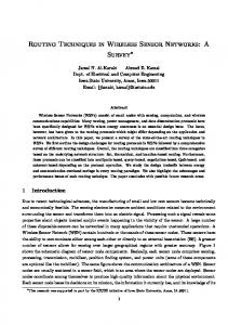
We consider a special family of networks (an example is provided in figure 1.1) whose behavior wrt the price of anarchy, as we shall see, is asymptotically equivalent to that of the parallel links model of [23] (which is actually a 1-layered network): Let ` ≥ 1 be an integer. A directed network G = (V, E) with a distinguished source–destination pair (s, t), s, t ∈ V , is an `-layered network if every (simple) directed s − t path has length exactly ` and each node lies on a directed s − t path. In a layered network there are no directed cycles and all directed paths are simple. In the following, we always use m = |E| to denote the number of edges in an `-layered network G = (V, E).

1.3

Related Work

1.3.1

Existence and Tractability of PNE

It is already known that the class of unweighted (atomic) congestion games (ie, players have the same demands and thus, the same affection on the resource delay functions) is guaranteed to have at least one PNE: actually, Rosenthal ([31]) proved that any potential game has at least one PNE and it is easy to write any unweighted congestion game as an exact potential game using Rosenthal’s potential function2 (eg, [12, Theorem 1]). In [12] it is proved that a PNE for any unweighted single–commodity network congestion game3 2 For

more details on potential games, see [29]. [12] only considers unit-demand players, this is also a symmetric network congestion game.

3 Since

1.3. RELATED WORK

9

(no matter what resource delay functions are considered, so long as they are non-decreasing with loads) can be constructed in polynomial time, by computing the optimum of Rosenthal’s potential function, through a nice reduction to min-cost flow. On the other hand, it is shown that even for a symmetric congestion game or an unweighted multi–commodity network congestion game, it is PLS-complete to find a PNE (though it certainly exists). The special case of single–commodity, parallel-edges network congestion game where the resources are considered to behave as parallel machines, has been extensively studied in recent literature. In [14] it was shown that for the case of players with varying demands and uniformly related parallel machines, there is always a PNE which can be constructed in polynomial time. It was also shown that it is NP-hard to construct the best or the worst PNE. In [17] it was proved that the fully mixed NE (FMNE), introduced and thoroughly studied in [27], is worse than any PNE, and any NE is at most (6 + ε) times worse than the FMNE, for varying players and identical parallel machines. In [26] it was shown that the FMNE is the worst possible for the case of two related machines and tasks of the same size. In [25] it was proved that the FMNE is the worst possible when the global objective is the sum of squares of loads. [13] studies the problem of constructing a PNE from any initial configuration, of social cost at most equal to that of the initial configuration. This immediately implies the existence of a PTAS for computing a PNE of minimum social cost: first compute a configuration of social cost at most (1+ε) times the social optimum ([18]), and consequently transform it into a PNE of at most the same social cost. In [11] it is also shown that even for the unrelated parallel machines case a PNE always exists, and a potential-based argument proves a convergence time (in case of integer demands) from arbitrary initial configuration to a PNE in time ³

´

O mWtot + 4Wtot /m+wmax . [28] studies the problem of weighted parallel-edges network congestion games with player– specific costs: each allowable action of a player consists of a single resource and each player has his own private cost function for each resource. It is shown that: (1) weighted (paralleledges network) congestion games involving only two players, or only two possible actions for all the players, or equal delay functions (and thus, equal weights), always possess a PNE; (2)

10


even a single–commodity, 3–players, 3–actions, weighted (parallel-edges network) congestion game may not possess a PNE (using 3-wise linear delay functions).

1.3.2

Price of Anarchy in Congestion Games

In the seminal paper [23] the notion of coordination ratio, or price of anarchy, was introduced as a means for measuring the performance degradation due to lack of players’ coordination when sharing common resources. In this work it was proved that the price of anarchy is 3/2 for two related parallel machines, while for m machines and players of varying demands, ´ ³√ ´ ³ m log m . For m identical parallel machines, [27] proved R = Ω logloglogmm and R = O that R = Θ

³

log m log log m

´

for the FMNE, while for the case of m identical parallel machines and

players of varying demands it was shown in [22] that R = Θ shown that R = Θ

³

log m log log log m

´

³

log m log log m

´

. In [9] it was finally

for the general case of related machines and players of varying

demands. [8] presents a thorough study of the case of general, monotone delay functions on parallel machines, with emphasis on delay functions from queuing theory. Unlike the case of linear cost functions, they show that the price of anarchy for non-linear delay functions in general is far worse and often even unbounded. In [32] the price of anarchy in a multi–commodity network congestion game among infinitely many players, each of negligible demand, is studied. The social cost in this case is expressed by the total delay paid by the whole flow in the system. For linear resource delays, the price of anarchy is at most 4/3. For general, continuous, non-decreasing resource delay functions, the total delay of any Nash flow is at most equal to the total delay of an optimal flow for double flow demands. [33] proves that for this setting, it is actually the class of allowable latency functions and not the specific topology of a network that determines the price of anarchy.

1.4. UNWEIGHTED CONGESTION GAMES

1.4

11

Unweighted Congestion Games

In this section we present some fundamental results connecting the classes of unweighted congestion games and (exact) potential games [29, 31]. Since we refer to players of identical (say, unit) weights, the players’ cost functions are λi ($) ≡

X

de (xe ($)) ,

ε∈$ i

where, xe ($) indicates the number of players willing to use resource e wrt configuration $ ∈ P. The following theorem proves the strong connection of congestion games with the exact potential games. Theorem 1.1 ([29, 31]) Every (unweighted) congestion game is an exact potential game. Proof: Fix an arbitrary (unweighted) congestion game Γ = (N, E, (P i )i∈N , (de )e∈E ). For any configuration $ ∈ P, consider the function Φ($) =

P e∈∪i∈N $ i

Pxe ($) k=1

de (k), which we

shall call Rosenthal’s potential. We can easily show that Φ is an exact potential for Γ: For this, consider arbitrary configuration $ ∈ P, an arbitrary player i ∈ N and an alternative (pure) strategy α ∈ P i \ {$i } for this player. Let also $ ˆ = $−i ⊕ α. Then, Φ($) ˆ − Φ($) =

ˆ e ($) X xX

de (k) −

e∈∪j $ ˆ j k=1

xe ($)+1

X



e∈∪i $ ˆ i \$ i

+

X e∈∪i

=

X

xe ($)

X

e∈$ î

de (k) −

k=1

de (xe ($)) ˆ −

X

de (k) 

de (k)

k=1

de (xe ($) + 1) −

e∈$ ˆ i \$i

=

de (k) −

X

xe ($)−1

X



xe ($) k=1



$i \$ î

X

k=1



de (k)

e∈∪j $j k=1



=

e ($) X xX

X

X

de (xe ($))

e∈$i \$ î

de (xe ($)) = λi ($) ˆ − λi ($)

e∈$i

where we have exploited the fact that ∀e ∈ E \ ($i ∪ $ ˆ i ) and ∀e ∈ $i ∩ $ ˆ i the load of each of these resources (ie, the number of players using them) remains the same. Additionally,

12


∀e ∈ $ ˆ i \ $i , xe ($) ˆ = xe ($) + 1 and ∀e ∈ $i \ $ ˆ i , xe ($) ˆ = xe ($) − 1. Remark 1.3 The existence of a (not necessarily exact) potential for any game in strategic form directly implies the existence of a PNE for this game. The existence of an exact potential may help (as we shall see later) the efficient construction of a PNE, but this is not true in general. More interestingly, Monderer and Shapley [29] proved that every (finite) potential game is isomorphic to an unweighted congestion game. The proof presented here is a new one provided by the authors of the survey. The main idea is based on the proof of Monderer and Shapley, yet it is much simpler and easier to follow. Theorem 1.2 ([29]) Every finite (exact) potential game is isomorphic to an unweighted congestion game. Proof:

Consider an arbitrary (finite) strategic game Γ = (N, (Y i )i∈N , (U i )i∈N ) among

n = |N | players, that admits an exact potential Φ : ×i∈N Y i 7→ R. Suppose that ∀i ∈ N, Y i = {1, 2, . . . , mi } ≡ [mi ] for some finite integer mi ≥ 2 (players having a unique allowable action can be safely removed from the game) and let Y ≡ ×i∈N Y i be the actions space of the game. We want to construct a proper unweighted congestion game C = (N, E, (P i )i∈N , (de )e∈E ) and a bijection $ : Y 7→ P (recall that P ≡ ×i∈N P i is the action space of C) such that ∀i ∈ N, ∀s ∈ Y, λi ($(s)) = U i (s) .

(1.6)

First of all, observe that for any (unweighted) congestion game C, we can express the players’ costs as follows: ∀i ∈ N, ∀$ ∈ P, λi ($) =

X

de (xe ($))

e∈$ i

=

X

e∈$ i ∩(E\∪j6=i $j )

+ ··· +

X

e∈∩k∈N

X

de (1) + e∈∪k6=i

de (n) $k

$i ∩$k ∩(E\∪

de (2) j6=i,k

$j )

(1.7)

1.4. UNWEIGHTED CONGESTION GAMES

13

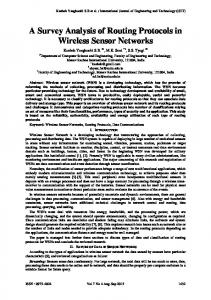
We proceed by determining the set of shared resources E = E1 ∪ E2 for our congestion game. We construct two sets of resources: The first set E1 contains resources that determine exactly what the players in the potential game actually do. The second set E2 contains resources that represent what all other players (except for the one considered by the resource) should not do. More specifically, fix an arbitrary configuration s ∈ Y of the players wrt the game Γ. We construct the following vector e(s) ∈ E1 which is nothing more than the binary representation of this configuration (see Figure 1.2):    1 k ∀k ∈ N, ∀j ∈ [mk ], ej (s) =   0,

if sk = j otherwise

Fix now an arbitrary player i ∈ N . We define n more resources whose binary vectors represent what the other players (ie, other than player i) in the potential game should not do (see Figure 1.3):    0 ∀k ∈ N, ∀j ∈ [mk ], ekj (s, i) =   1,

if k 6= i and sk = j otherwise

It is easy to see that e(s, i) actually says that none of the players k 6= i agrees with the profile s−i ∈ Y −i . So, we force this binary vector e(s, i) to have definitely 0s exactly at the positions where s−i has 1s for any of the players except for player i, and we place 1s anywhere else. For m = m1 + m2 + · · · + mn , let E1 = {e(s) ∈ {0, 1}m : s ∈ Y } and E2 = {e(s, i) ∈ {0, 1}m : (i ∈ N ) ∧ (s−i ∈ Y −i )}. The set of resources in our congestion game is then E = E1 ∪ E2 . We now proceed with the definition of the action sets of the players wrt C. Indeed, i }, where ∀j ∈ [mi ], πji = {e ∈ E : eij = 1}. Now the bijective map ∀i ∈ N, P i = {π1i , . . . , πm i

that we assume is almost straightforward: ∀s = (si )i∈N ∈ Y, $(s) = (πsi i )i∈N . Some crucial observations are the following: First, ∀s ∈ Y , the resource e(s) is the only resource in E1 that is used by all the players when the configuration $(s) is considered. For any other configuration z ∈ Y \ {s}, the resource e(s) is not used by at least one player, assuming $(z). Similarly, ∀s ∈ Y, ∀i ∈ N , the resource e(s, i) is the only resource in E2

14


that is exclusively used by player i, assuming the configuration $(s). Now it is very simple to set the resource delay functions de in such a way that we assure equality (1.6). Indeed, observe that ∀i ∈ N, ∀s ∈ Y, ∀α ∈ Y i \ {si }, U i (s) − U i (s−i ⊕ α) = Φ(s) − Φ(s−i ⊕ α) ⇔ Qi (s−i ) ≡ U i (s) − Φ(s) = U i (s−i ⊕ α) − Φ(s−i ⊕ α) . That is, the quantity Qi (s−i ) is invariant of player i’s strategy. Recall the form of player i’s cost given in equality (1.7). The charging scheme of the resources that we adopt is as follows: ∀e ∈ E, de (k) =

   Qi (s−i ),   

0,      Φ(s),

if (k = 1) ∧ (e = e(s, i) ∈ E2 ) if (1 < k < n) ∨ (k = 1 ∧ e ∈ E1 ) if (k = n) ∧ (e = e(s) ∈ E1 )

Now it is easy to see that for any player i ∈ N and any configuration s ∈ Y , the only resource used exclusively by i wrt to s which has non-zero delay, is e(s, i). Similarly, the only resource used by all the players that has non-zero delay is e(s). All other resources charge zero delays, no matter how many players use them. Thus, ∀i ∈ N, ∀s ∈ Y, (1.7) ⇒ λi ($(s)) = de(s,i) (1) + de(s) (n) = Qi (s−i ) + Φ(s) = U i (s) .

Remark 1.4 The size of the congestion game that we use to represent a potential game is at most (|N | + 1) times larger than the size of the potential game. Since an unweighted congestion game is itself an exact potential game, this implies an essential equivalence of exact potential and unweighted congestion games.

1.5. EXISTENCE AND COMPLEXITY OF CONSTRUCTING PNE

1.5

15

Existence and Complexity of Constructing PNE

In the present section we deal with issues concerning the existence and complexity of constructing PNE in weighted congestion games. Our main references for this section are [12, 15, 24]. We start with some complexity issues concerning the construction of PNE in unweighted congestion games (in which a PNE always exists) and consequently we study existence and complexity issues in weighted congestion games in general. Fix an arbitrary (weighted in general) congestion game Γ = (N, E, (P i )i∈N , (wi )i∈N , (de )e∈E ) where the wi ’s denote the (positive) weights of the players. A crucial class of problems containing the weighted network congestion games is PLS [21] (stands for Polynomial Local Search). This is the subclass of total functions in NP that are guaranteed to have a solution because of the fact that “every finite directed acyclic graph has a sink”. A local search problem Π has a set of instances DΠ which are strings. To each instance x ∈ DΠ , there corresponds a set SΠ (x) of solutions, and a standard solution s0 ∈ SΠ (x). Each solution s ∈ SΠ (x) has a cost fΠ (s, x) and a neighborhood NΠ (s, x). The search problem is, given an instance x ∈ DP i , to find a locally optimal solution s ∈ SΠ (x), ie, a solution s∗ ∈ SΠ (x) s.t. fΠ (s∗ , x) = maxs∈NΠ (s∗ ,x) {fΠ (s, x)} (assuming that we consider as our objective the minimization of the cost function). Definition 1.1 (Polynomial Local Search (PLS)) A local search problem Π is in PLS if its instances DΠ and solutions SΠ (x : x ∈ DΠ ) are binary strings, there is a polynomial p such that the length of solutions SΠ (x) is bounded by p(|x|), and there are three polynomial– time algorithms AΠ , BΠ , CΠ with the following properties: 1. Given a string x ∈ {0, 1}∗ , AΠ determines whether x ∈ DΠ , and if so, returns some initial solution s0 ∈ SΠ (x). 2. Given an instance x ∈ DΠ and a string s, BΠ determines whether s ∈ SΠ (x), and if so, computes the value fΠ (s, x) of the cost function at s. 3. Given an instance x ∈ DΠ and a solution s ∈ SΠ (x), CΠ determines whether s is a

16

CHAPTER 1. ATOMIC SELFISH ROUTING IN NETWORKS: A SURVEY local optimum of fΠ (·, x) in its neighborhood NΠ (s, x), and if not, returns a neighbor s0 ∈ NΠ (s, x) having a better value (ie, fΠ (s0 , x) < fΠ (s, x) for a minimization problem and fΠ (s0 , x) > fΠ (s, x) for a minimization problem). The problem of constructing a PNE for a weighted congestion game is in PLS, in the

following cases: (1) for any unweighted congestion game, since it is an exact potential game (see Theorem 1.1), and (2) for any weighted network congestion game with linear resource delays, which admits (as we shall prove in Theorem 1.6) a b−potential with bi =

1 , ∀i 2wi

∈ N,

and thus finding PNE is equivalent to finding local optima for the optimization problem with state space the action space of the game and objective the potential of the game. On the other hand, this does not imply a polynomial-time algorithm for constructing a PNE, since (as we shall see more clearly in the weighted case) the improvements in the potential can be very small and too many. Additionally, although problems in PLS admit a PTAS, this does not imply also a PTAS for finding ε-approximate PNE (approximation of the potential does not imply also approximation of each player’s payoff).

1.5.1

Efficient Construction of PNE in Unweighted Congestion Games

In this subsection we shall prove that for unweighted single–commodity network congestion games a PNE can be constructed in polynomial time. On the other hand, even for multi– commodity network congestion games it is PLS complete to construct a PNE. The main source of this subsection is the work of Fabrikant, Papadimitriou and Talwar [12]. Theorem 1.3 ([12]) There is a polynomial time algorithm for finding a PNE in any unweighted single–commodity network congestion game. Proof:

Fix an arbitrary unweighted, single–commodity network congestion game Γ =

(N, E, (Ps−t )i∈N , (de )e∈E ) and let G = (V, E) be the underlying network. Recall that this game admits Rosenthal’s exact potential Φ($) =

P e∈E

Pxe ($) k=1

de (k). The algorithm com-

putes the optimum value of Φ : P 7→ R in the action space of the game. The corresponding configuration is thus a PNE.


17

The algorithm exploits a reduction to a min-cost flow problem. This reduction is done as follows: We construct a new network G0 = (V 0 , E 0 ) with the same set of vertices V 0 = V , while the set of arcs (ie, resources) is defined as follows (see also Figure 1.4): ∀e = (u, v) ∈ E, we add n parallel arcs from u to v, e0 (1), . . . , e0 (n) ∈ E, where these arcs have a capacity of 1 (ie, they allow at most one player to use each of them) and fixed delays (when used) |E 0 |

∀k ∈ [de (n)], d0e0 (k) = de (k). Let f ∗ ∈ R≥0 be a minimizer of the following min-cost flow problem: min

X

d0e0 · fe0

e0 ∈E 0

s.t.

X

fe0 − fe0 −

e0 =(u,t)∈E 0

∀v ∈ V \ {s, t},

X

X

f e0 = n

e0 =(t,u)∈E 0

f e0 =

e0 =(v,u)∈E 0

∀e0 ∈ E 0 ,

f e0 = n

e0 =(u,s)∈E 0

e0 =(s,u)∈E 0

X

X

X

f e0

e0 =(u,v)∈E 0

0 ≤ f e0 ≤ 1

This problem can be solved in polynomial time [1] (eg, in time O(r log k(r + k log k)) using scaling algorithms) where r = |E 0 | = |E| · n and k = |V | are the number of arcs and the number of nodes in the underlying (augmented) network respectively. It is straightforward to see that any min-cost flow in G0 is integral and it corresponds to a configuration in Γ that minimizes the potential of the game (which is then a PNE). On the other hand, the following theorem proves that it is not that easy to construct a PNE, even in an unweighted multi–commodity network congestion game. We give this theorem with a sketch of its proof:

Theorem 1.4 ([12]) It is PLS-complete to find a PNE in unweighted congestion games of the following types: (i) General congestion games, (ii) symmetric congestion games, and (iii) multi–commodity network congestion games.

18


Proof: We only give a sketch of the first two cases. The PLS completeness proof of case (iii) is rather complicated and therefore is not presented in this survey. The interested reader may find it in [12]. We first prove the PLS completeness of general congestion games and consequently we show that an arbitrary congestion game can be transformed into an equivalent symmetric congestion game. In order to prove the PLS completeness of a congestion game, we shall use the following problems:

NOTALLEQUAL3SAT: Given a set N of {0, 1}−variables and a collection C of clauses s.t. ∀c ∈ C, |c| ≤ 3, is there an assignment of values to the variables so that no clause has all its literals assigned the same value?

POSNAE3FLIP: Given an instance (N, C) of NOTALLEQUAL3SAT with positive literals only and a weight function w : C 7→ R, find an assignment for the variables of N , s.t. the total weight of the unsatisfied clauses and the totally satisfied (ie, with all their literals set to 1) clauses cannot be decreased by a unilateral flip of the value of any variable.

It is known that POSNAE3FLIP is PLS complete [34].Given an instance of POSNAE3FLIP, we shall construct a congestion game Γ = (N, E, (P v )v∈N , (de )e∈E ) as follows: The player set of the game is exactly the set of variables N . ∀c ∈ C, we construct two resources ec , e0c ∈ E whose delay functions are de (k) = w(c) · I{k=3} and de0 (k) = w(c) · I{k=3} . That is, resource ec (or e0c ) has delay w(c) only when all the 3 players it contains actually use it. Each player v ∈ N has exactly two allowable actions indicating the possible true (ie, 1) or false (ie, 0) values of the corresponding variable: P v = {{ec ∈ E : v ∈ c}, {e0c ∈ E : v ∈ c}}. Smaller clauses (ie, of two literals) are implemented similarly. Clearly, a flip of a variable corresponds to the change in the strategy of the corresponding player. The changes in the total weight due to a flip equal the changes in the cumulative delay over all the resources. Thus, any PNE of the congestion game Γ is a local optimum (ie, a solution) of the POSNAE3FLIP problem, and vice versa.


19

We now proceed to show that any unweighted congestion game can be transformed into a symmetric congestion game. Let Γ = (N, E, (P v )v∈N , (de )e∈E ) be an arbitrary congestion ³ ´ ˆ = N, E, ˆ P, ˆ (dê ) ˆ as game. We construct an equivalent symmetric congestion game Γ e∈E

follows: First of all we add to the set of resources n new distinct resources: Eˆ = E ∪ {ei }i∈N . The delays of these resources are: ∀i ∈ N, dê (k) = M · I{k≥2} for some sufficiently large i

constant M . The old resources maintain the same delay functions: ∀e ∈ E, ∀k ≥ 0, dê (k) = de (k). Now each player has the same action set Pˆ = ×i∈N {a ∪ {ei } : a ∈ P i }. Observe that ˆ each of the distinct resources (by setting the constant M sufficiently large) in any PNE of Γ {ei }i∈N is used by exactly one player (these resources act as if they have capacity 1 and ˆ we can easily get a PNE in Γ by simply there are only n of them). So, for any PNE in Γ dropping the unique new resource used by each of the players. This is done by identifying ˆ according to the unique resource they use, and match them the “anonymous” players of Γ with the corresponding players of Γ.

1.5.2

Existence and Construction of PNE in Weighted Congestion Games

In this Section we deal with the existence and tractability of PNE in weighted network congestion games. First we show that it is not always the case that a PNE exists, even for a weighted single–commodity network congestion game with only linear and 2-wise linear (ie, the maximum of two linear functions) resource delays. Recall that, as discussed previously, any unweighted congestion game has a PNE, for any kind of non-decreasing delays, due to the existence of an exact potential for these games. This result was independently proved by [15] and [24], based on similar constructions. In this survey we present the version of [15] due to its clarity and simplicity. Lemma 1.1 ([15]) There exist instances of weighted single–commodity network congestion games with resource delays being either linear or 2-wise linear functions of the loads, for which there is no PNE.

Proof:

We demonstrate this by the example shown in Figure 1.5.

In this example

there are exactly two players of demands w1 = 1 and w2 = 2, from node s to node

20


t. The possible paths that the two players may follow are labeled in the figure. The resource delay functions are indicated by the 3 possible values they may take given the two players. Observe now that this example has no PNE: there is a simple closed path γ = ((P 3, P 2), (P 3, P 4), (P 1, P 4), (P 1, P 2), (P 3, P 2)) of length 4 that is an improvement path (actually, each defecting player moves to his new best choice, so this is a best–reply improvement path) and additionally, any other configuration not belonging to γ is either one, or two best–reply moves away from some of these nodes. Therefore there is no sink in the Nash Dynamics Graph of the game and thus there exists no PNE. Observe that the delay functions are not player–specific in our example, as was the case in [28]. Consequently we show that there may exist no exact potential function for a weighted single–commodity network congestion game, even when the resource delays are identical to their loads. The next argument shows that Theorem 1.1 does not hold anymore even in this simplest case of weighted congestion games.

Lemma 1.2 ([15]) There exist weighted single–commodity network congestion games which are not exact potential games, even when the resource delays are identical to their loads.

Proof: Let Γ = (N, E, (wi )i∈N , (P i )i∈N , (de )e∈E ) denote a weighted single–commodity network congestion game with de (x) = x, ∀e ∈ E. Recall the definition of players’ costs for a configuration (Eq. (1.1)). Let’s now define, for any path γ = ($(0), . . . , $(r)) in the configuration space P of Γ, the quantity I(γ, λ) =

Pr

k=1

[λik ($(k)) − λik ($(k − 1))], where ik is

the unique player in which the configurations $(k) and $(k − 1) differ. Our proof is based on the fact that Γ is an (exact) potential game if and only if every simple closed path γ of length 4 has I(γ, λ) = 0 ([29, Theorem 2.8]). For the sake of contradiction, assume that every closed simple path γ of length 4 for Γ has I(γ, λ) = 0, fix arbitrary configuration $ and consider the path γ = ($, x = $−1 ⊕ π1 , y = $−(1,2) ⊕ (π1 , π2 ), z = $−2 ⊕ π2 , $) for some actions π1 6= $1 and π2 6= $2 . We shall demonstrate that I(γ, λ) cannot be identically 0 when there are at least two players of different demands. So, consider that the first two players have different demands: w1 6= w2 .


21

We observe that λ1 (x) − λ1 ($) =

X

θe (x) −

e∈π1

X

θe ($)

e∈$1

= |π1 \ $1 | · w1 +

X

X

θe ($) −

e∈π1 \$1

θe ($)

e∈$1 \π1

since the resources in $1 ∩ π1 retain their initial loads. Similarly we have: λ2 (y) − λ2 (x) =

X e∈π2

\$2

= |π2 \ $2 | · w2 + λ1 (z) − λ1 (y) =

X X

e∈$1 \π1

λ2 ($) − λ2 (z) =

X

X X

θe (z) −

θe (x)

e∈$2 \π2

θe (x) −

e∈π2 \$ 2

e∈$1 \π1

=

X

[θe (x) + w2 ] −

X

θe (x)

e∈$2 \π2

[θe (z) + w1 ]

e∈π1 \$1

X

θe (z) −

θe (z) − |π1 \ $1 | · w1

e∈π1 \$1

θe ($) −

e∈$2 \π2

X

θe ($) − |π2 \ $2 | · w2

e∈π2 \$ 2

Thus, since I ≡ I(γ, λ) = λ1 (x) − λ1 ($) + λ2 (y) − λ2 (x) + λ1 (z) − λ1 (y) + λ2 ($) − λ2 (z), we get: I =

X

[θe ($) − θe (z)] +

e∈π1 \$1

+

X

e∈$ 1 \π1

X

[θe (x) − θe ($)] +

e∈π2 \$ 2

[θe (z) − θe ($)] +

X

[θe ($) − θe (x)]

e∈$2 \π2

Observe now that ∀e ∈ π1 \ $1 ,

³

´

³

´

³

´

θe ($) − θe (z) = θe ($) − θe ($−2 ⊕ π2 ) = w2 · I{e∈$2 \π2 } − I{e∈π2 \$2 } ∀e ∈ π2 \ $2 ,

θe (x) − θe ($) = θe ($−1 ⊕ π1 ) − θe ($) = w1 · I{e∈π1 \$1 } − I{e∈$1 \π1 } ∀e ∈ $1 \ π1 ,

θe (z) − θe ($) = θe ($−2 ⊕ π2 ) − θe ($) = w2 · I{e∈π2 \$2 } − I{e∈$2 \π2 }

22

CHAPTER 1. ATOMIC SELFISH ROUTING IN NETWORKS: A SURVEY ∀e ∈ $2 \ π2 ,

³

θe ($) − θe (x) = θe ($) − θe ($−1 ⊕ π1 ) = w1 · I{e∈$1 \π1 } − I{e∈π1 \$1 }

´

Then, I = (w1 − w2 ) ·

h

|(π1 \ $1 ) ∩ (π2 \ $2 )| + |($1 \ π1 ) ∩ ($2 \ π2 )|−

−|($1 \ π1 ) ∩ (π2 \ $2 )| − |(π1 \ $1 ) ∩ ($2 \ π2 )|

i

,

which is typically not equal to zero for a single–commodity network. It should be noted that the second parameter, which is network dependent, can be non-zero even for some cycle of a very simple network. For example, in the network of Figure 1.5 (which is a simple 2-layered network) the simple closed path γ = ($(0) = (P 1, P 3), $(1) = (P 2, P 3), $(2) = (P 2, P 1), $(3) = (P 1, P 1), $(4) = (P 1, P 3)) has this quantity equal to −4 and thus no weighted single–commodity network congestion game on this network can admit an exact potential. Our next step is to focus our interest on the `-layered networks with resource delays identical to their loads. We shall prove that any weighted `-layered network congestion game with these delays admits at least one PNE, which can be computed in pseudo-polynomial time. Although we already know that even the case of weighted `-layered network congestion games with delays equal to the loads cannot have any exact potential4 , we will next show that Φ($) ≡

P

e∈E [θe ($)]

2

is a b-potential for such a game and some positive n-vector b,

assuring the existence of a PNE. Theorem 1.5 ([15]) For any weighted `-layered network congestion game with resource delays equal to their loads, at least one PNE exists and can be computed in pseudo-polynomial time. Proof: Fix an arbitrary `-layered network (V, E) and denote by L all the s − t paths in it from the unique source s to the unique destination t. Let $ ∈ P ≡ Ln be an arbitrary configuration of the players for the corresponding congestion game on (V, E). Also, let i be 4 The

example at the end of the proof of lemma 1.2 involves the 2-layered network of Figure 1.5.


23

a user of demand wi and fix some path α ∈ L. Denote $ ˆ ≡ $−i ⊕ α. Observe that X³

Φ($) − Φ($) ˆ = =

X ³

´

θe2 ($) − θe2 ($) ˆ

e∈E

θe2 ($)

´

− θe2 ($) ˆ +

e∈$ i \α

=

X ³

=

´

θe2 ($) − θe2 ($) ˆ

e∈α\$i

´

X ³

[θe ($−i ) + wi ]2 − θe2 ($−i ) +

e∈$ i \α

X ³

X ³

´

X ³

wi2 + 2wi θe ($−i ) −

e∈$ i \α

θe2 ($−i ) − [θe ($−i ) + wi ]2

e∈α\$i

´

wi2 + 2wi θe ($−i )

e∈α\$ i

³



´

= wi2 · |$i \ α| − |α \ $i | + 2wi ·  = 2wi · 

 X

θe ($−i ) −

e∈$i \α





X

θe ($−i ) −

e∈$i \α

X

´

X

θe ($−i )

e∈α\$ i

h

i

θe ($−i ) = 2wi · λi ($) − λi ($) ˆ ,

e∈α\$ i

since, ∀e ∈ $i ∩ α, θe ($) = θe ($), ˆ in `-layered networks |$i \ α| = |α \ $i |, λi ($) = P e∈$ i

θe ($) =

P

e∈α\$ i

P

e∈$i \α θe ($

−i

θe ($−i ) + wi |α \ $i | +

) + wi |$i \ α| +

P

e∈$ i ∩α θe ($).

P

e∈$i ∩α θe ($)

and λi ($) ˆ =

P

ˆ e∈α θe ($)

=

Thus, Φ is a b−potential for our game, where

b = (1/(2wi ))i∈N ∈ Rn>0 , assuring the existence of at least one PNE. We proceed with the construction of a PNE in pseudopolynomial time. Wlog assume now that the players have integer weights. Then each player performing any improving defection, must reduce his cost by at least 1 and thus the potential function decreases by at least 2wmin ≥ 2 along each arc of the Nash Dynamics Graph of the game. Consequently, the na¨ıve algorithm that, starting from an arbitrary initial configuration $ ∈ P, follows any improvement path that leads to a sink (ie, a PNE) of the Nash Dynamics Graph, cannot 2 2 . defections, since ∀$ ∈ P, Φ($) ≤ |E|Wtot contain more than 21 |E|Wtot

A recent improvement, based essentially on the same technique as above, generalizes the last result to the case of arbitrary multi–commodity network congestion games with linear resource delays (we state the result here without its proof):

Theorem 1.6 ([16]) For any weighted multi–commodity network congestion game with linear resource delays, at least one PNE exists and can be computed in pseudo-polynomial time.

24


1.6

Parallel Links and Player Specific Payoffs

In [28] Milchtaich studies a variant of the classical (unweighted) congestion games, where the resource delay functions are not universal, but player–specific. In particular, there is again a set E of shared resources and a set N of (unit–demand) players with their action sets (Pi )i∈N , but rather than having a single delay de : R≥0 7→ R per resource e ∈ E, there is actually a different utility function5 per player i ∈ N and resource e ∈ E, Uei : R≥0 7→ R determining the payoff of player i for using resource e, given a configuration $ ∈ P and the load θe ($) induced by it on that resource. On the other hand, Milchtaich makes two simplifying (yet crucial) assumptions: (1) each player may choose only one resource from a pool E of resources (shared to all the players) for his service (ie, this is modeled as the parallel-links model of Koutsoupias and Papadimitriou [23]), and (2) the received payoff is monotonically non-increasing with the number of players selecting it. Although they do not always admit a potential, these games always possess a PNE. In [28] Milchtaich proved that unweighted congestion games on parallel links with player– specific payoffs, involving only two strategies, possess the Finite Improvement Property (FIP). It is also rather straightforward that any 2–players unweighted congestion game on parallel links with player–specific payoffs possesses the Finite Best Reply improvement path Property (FBRP). Milchtaich also gave an example of an unweighted congestion game on three parallel links with three players, for which there is a best–reply cycle (although there is a PNE). The example is shown in Figure 1.6. In this example, we only determine the necessary conditions on the (player–specific) payoff functions of the players for the existence of the best-response cycle (see figure). It is easily verified that this system of inequalities is feasible, and that configurations (3, 1, 2) and (2, 3, 1) are PNE for the game. 5 In this case we refer to the utility of a player, that each player wishes to maximize rather than minimize. Eg, this is the negative of a player’s private cost function on a resource.

1.6. PARALLEL LINKS AND PLAYER SPECIFIC PAYOFFS

25

Theorem 1.7 ([28]) Every unweighted congestion game on parallel links with player–specific, non-increasing payoffs of the resources, possesses a PNE.

Proof:

First of all, we need to prove the following lemma that bounds the lengths of

best–reply paths of a specific kind. Lemma 1.3 Let (e(0), e(1), . . . , e(M )) be a sequence of (possibly repeated) resources from E. type–(a) path: Let ($(1), $(2), . . . , $(M )) be a best–reply improvement path of the game, s.t. ∀t ≥ 1, ∀e ∈ E,    xe (t − 1),   

xe (t) =  xe (t − 1) + 1,

    xe (t − 1) − 1,

if e ∈ / {e(t − 1), e(t)} if e = e(t) if e = e(t − 1)

Then M ≤ |N |. type–(b) path: Let ($(1), $(2), . . . , $(M )) be a best–reply improvement path of the game, s.t. ∀t ≥ 1, ∀e ∈ E,

xe (t) =

   xe (t − 1),   

xe (t − 1) + 1,      xe (t − 1) − 1,

if e ∈ / {e(t − 1), e(t)} if e = e(t − 1) if e = e(t)

Then, M ≤ |N | · (|E| − 1).

Proof: (a) Fix a best–reply, type–(a) improvement path γ = ($(1), $(2), . . . , $(M )) (see ≡ min0≤t≤M {xe (t)} denote the minimum (a) of Figure 1.7). For each resource e ∈ E, let xmin e load of e among the configurations involved in γ. By definition of γ as a best–reply sequence, + 1. That is, a resource we observe that ∀e ∈ E, ∀t ≥ 1, xe(t) (t) = xe(t) (t − 1) + 1 = xmin e reaches its maximum load exactly when it is the unique node in γ that currently receives a new player, reaches its minimum load in the very next time step (because of losing a player),

26


and remains at its minimum load until before it appears again in this sequence. But then, the unique deviator in each move goes to a resource that reaches its maximum load, whereas all the other resources are already at their minimum loads. This implies that there is no chance that the specific player will move away from this new resource that he selfishly chose, till the end of the best–reply path under consideration. More formally, ∀t ≥ 1, let i(t) be the unique deviator that moves from e(t − 1) to e(t). Then, ∀t ∈ [M ], we can verify (by induction on t0 ) that ∀t + 1 ≤ t0 ≤ M, ∀e ∈ E \ {e(t)}, i(t)

i(t)

³

´

´

³

i(t) Ue(t) (xe (t0 )) ≥ Ue(t) xmin xmin + 1 ≥ Uei(t) (xe (t0 ) + 1) e e(t) + 1 ≥ Ue

and so, i(t) will not selfishly move away from e(t) till the end of the best–reply improvement path. The first and the third inequality are true because of the monotonicity of the payoff functions. The second inequality is due to the selfish choice (by player i(t)) of resource e(t) at time t, despite the fact that e(t) reaches its maximum load and all the other resources have their minimum loads after this move. Since this holds for all players, this path may have length at most |N |. (b) Fix now a best–reply, type–(b) improvement path γ = ($(1), $(2), . . . , $(M )) (see (b) of Figure 1.7). For each resource e ∈ E, let again xmin ≡ min0≤t≤M xe (t). We observe e min that ∀1 ≤ t ≤ M, xe(t) (t) = xmin e(t) and xe(t−1) (t) = xe(t−1) + 1. Due to the best–reply moves

considered in the path, if i(t) is again the unique deviator from e(t) towards e(t − 1) at time t, then ∀1 ≤ t ≤ M , i(t)

³

´

i(t)

³

´

Ue(t) xe(t) (t − 1) = Ue(t) xmin e(t) + 1 < i(t)

³

´

i(t)

³

< Ue(t−1) xe(t−1) (t − 1) + 1 = Ue(t−1) xmin e(t−1) + 1

´

which implies that ∀t0 > t player i(t) residing at a resource e 6= e(t) could never prefer to deviate to e(t) rather than deviate to (or, stay at, if already there) resource e(t − 1). That is, player i(t) can never go back to the resource from which it defected once, till the end of the best–reply path. Thus, each player can make at most |E| − 1 moves and so, M ≤ |N | · (|E| − 1).

1.6. PARALLEL LINKS AND PLAYER SPECIFIC PAYOFFS

27

The proof of the theorem proceeds by induction on the number of players. Trivially, for a single player we know that as soon as he is at a best reply, this is also a PNE (there is nothing else to move). We assume now that any unweighted congestion game on parallel ³ ´ ˜ | < n, Γ ˜ = N ˜ , E, (U i ) ˜ links with player–specific payoffs and |N e i∈N ,e∈E , possesses a PNE. We want to prove that this is also the case for any such game with n players. Let N = [n] and Γ = (N, E, (Uei )i∈N,e∈E ) be such a game. We temporarily pull player n out of the game and let the remaining n − 1 players continue playing, until they reach a PNE (without player ³ ´ ˜ = [n − 1], E, (Uei )i∈[n−1] , e ∈ E n) s ∈ E n−1 . That the PNE s exists for the pruned game Γ holds by inductive hypothesis. Now we let player n be assigned to a best–reply resource e ∈ BRn (s), and we thus construct a configuration $(0) as follows: $n (0) = e; ∀i ∈ [n − 1], $i (0) = si . Consequently, starting from $(0), we construct a best–reply maximal improvement path of type (a) (see previous lemma) Π(a) = ($(0), $(1), . . . , $(M )), which we already know that is of length at most n. We claim that the terminal configuration of this path is a PNE for Γ. Clearly, any player that deviated to a best–reply resource in Π(a) does not move again and is also at a best–reply resource in $(M ) (see the proof of the lemma). So we only have to consider players that have not defected during Π(a). Fix any such player i, residing at resource e = $i (0) = si . Observe that in $(M ) the following holds:

∀e ∈ E, xe (M ) =

   xe (0),

if e 6= e(M ),

  xe (0) + 1,

if e = e(M )

Observe that if some player i : si (M ) = e(M ) that has not moved during Π(a) is not at his best reply in $(M ), then we can set e(M + 1) ∈ BRi ($−i (M )) and thus augment the best–reply improvement path Π(a), which contradicts the maximality assumption. Consider now any player i ∈ e 6= e(M ) that has not moved during Π(a). This player is certainly at a best–reply resource e ∈ BRi ($−i (M )) since this resource has exactly the same load as in s and any other resource has at least the load it had in s. So, $(M ) is a PNE for Γ since every player is at a best–reply resource wrt $(M ). This completes the proof of the theorem.

28


Remark 1.5 Observe that the proof of this theorem is constructive, and thus also implies a path of length at most |N | that leads to a PNE. But this is not necessarily an improvement path, when all players are considered to coexist all the time, and therefore there is no justification of the adoption of such a path by the (selfish) players. Milchtaich [28], using an argument of the same flavor as in the above theorem, proves that from an arbitrary initial configuration and allowing defections, there is a best–reply improvement path   only best–reply |N | + 1  . The idea is, starting from an arbitrary configuration 2 $(0), to let the players construct a best–reply improvement path of type–(a), and then (if of length at most |E| ·  

necessary) construct a best–reply improvement path of type–(b) starting from the terminal configuration of the previous path. It is then easily shown that the terminal configuration of the second path is a PNE of the game. The unweighted congestion games on parallel links and with player–specific payoffs are weakly acyclic games, in the sense that from any initial configuration $(0) of the players, there is at least one best–reply improvement path connecting it to a PNE. Of course, this does not exclude the existence of best–reply cycles (see example of Figure 1.6). But, it is easily shown that when the deviations of the players occur sequentially and in each step the next deviator is chosen randomly (among the potential deviators) to a randomly chosen best–reply resource, then this path will converge almost surely to a PNE in finite time.

1.6.1

Players with Distinct Weights

Milchtaich proposed a generalization of his variant of congestion games, by allowing the players to have distinct weights, denoted by a weight vector w = (w1 , w2 , . . . , wn ) ∈ Rn>0 . In that case, the (player–specific) payoff of each player on a resource e ∈ E depends on the load θe ($) ≡

P i:e∈$ i

wi , rather than the number of players willing to use it.

For the case of weighted congestion games on parallel links with player specific payoffs, it is easy to verify (in a similar fashion as for the unweighted case) that: • If there are only two available strategies then FIP holds.

1.7. THE PRICE OF ANARCHY OF WEIGHTED CONGESTION GAMES

29

• If there are only two players then FBRP holds. • For the special case of resource specific payoffs, FIP holds.

On the other hand, there exists a 3–players, 3–actions game that possesses no PNE. For example, see the instance shown in Figure 1.8, where the three players have essentially two strategies each (a “LEFT” and a “RIGHT” strategy) to choose from, while their third strategies give them strictly minimal payoffs and can never be chosen by selfish moves. The rationale of this game is that, in principle, player 1 would like to avoid using the same link as player 3, which in turn would like to avoid using the same link as player 2, which would finally want to avoid player 1. The inequalities shown in Figure 1.8(b) demonstrate the necessary conditions for the existence of a best–reply cycle among 6 configurations of the players. It is easy to verify also that any other configuration has either at least one MIN strategy for some player (and in that case this player wants to defect) or is one of (2, 2, 1), (3, 3, 3). The only thing that remains to assure, is that (2, 3, 1) is strictly better for player 2 than (2, 2, 1) (ie, player 2 would like to avoid player 1) and that (3, 3, 1) is better for player 3 than (3, 3, 3) (ie, player 3 would like to avoid player 2). The feasibility of the whole system of inequalities can be trivially checked to hold, and thus this game cannot have any PNE since there is no sink in its Dynamics graph.

1.7

The Price of Anarchy of Weighted Congestion Games

In this section we focus our interest on weighted `-layered network congestion games where the resource delays are identical to their loads. Our source for this section is [15]. This case comprises a highly non-trivial generalization of the well–known model of selfish routing of atomic (ie, indivisible) traffic demands via identical parallel channels [23]. The main reason why we focus on this specific category of resource delays is that there exist instances of (even unweighted) congestion games on layered networks that have unbounded price of anarchy even if we only allow linear resource delays. In [32, p. 256] an example is given where the price

30


of anarchy is indeed unbounded (see Figure 1.9). This example is easily converted into an `-layered network. The resource delay functions used are either constant, or M/M/1-like (ie, of the form

1 ) c−x

delay functions. However, we can be equally bad even with linear resource

delay functions: Observe the following example depicted in Figure 1.10. Two players, each having a unit of traffic demand from s to t, choose their selected paths selfishly. The edge delays are shown above them in the usual way. We assume that a À b À 1 ≥ c. It is easy to see that the configuration (sCBt,sADt) is a PNE of social cost 2 + b while the optimum configuration is (sABt,sCDt) the (optimum) social cost of which is 2 + c. Thus, R =

b+2 . c+2

In the following, we restrict our attention to `-layered networks whose resource delays are equal to their loads. Our main tool is to interpret a strategies profile as a flow in the underlying network.

1.7.1

Flows and Mixed Strategies Profiles

Fix an arbitrary `-layered network G = (V, E) and a set N = [n] of distinct players willing to satisfy their own traffic demands from the unique source s ∈ V to the unique destination t ∈ V . Again, w = (wi )i∈[n] denotes the varying demands of the players. Fix an arbitrary mixed strategies profile p = (p1 , p2 , . . . , pn ) where, for sake of simplicity, we consider that ∀i ∈ [n], pi : Ps−t 7→ [0, 1] is a real function (rather than a vector) assigning non-negative probabilities to the s − t paths of G (which are the allowable actions for player i). A feasible flow for the n players is a function ρ : Ps−t 7→ R≥0 mapping amounts of non-negative traffic (on behalf of all the players) to the s − t paths of G, in such a way that P π∈Ps−t

ρ(π) = Wtot ≡

P i∈[n]

wi . That is, all players’ demands are actually satisfied. We

distinguish between unsplittable and splittable (feasible) flows. A feasible flow is unsplittable if each player’s traffic demand is satisfied by a unique path of Ps−t . In the general case, any feasible flow is splittable, in the sense that the traffic demand of each player is possibly routed over several paths of Ps−t . We map the mixed strategies profile p to a feasible flow ρp as follows: For each s − t path π ∈ Ps−t , ρp (π) ≡

P i∈[n]

wi · pi (π). That is, we handle the expected load traveling along


31

π according to p as a splittable flow, where player i routes a fraction of pi (π) of his total demand wi along π. Observe that, if p is actually a pure strategies profile, the corresponding flow is then unsplittable. Recall now that for each edge e ∈ E, θe (p) =

n X X

wi pi (π) =

X

ρp (π) ≡ θe (ρp )

π:e∈π

i=1 π:e∈π

denotes the expected load (and in our case, also the expected delay) of e wrt p, and can be expressed either as a function θe (p) of the mixed profile p, or as a function θe (ρp ) of its associated feasible flowρp . As for the expected delay along a path π ∈ Ps−t according to p, this is θπ (p) =

X

θe (p) =

e∈π

XX

ρp (π 0 ) =

e∈π π 0 3e

X

|π ∩ π 0 |ρp (π 0 ) ≡ θπ (ρp ) .

π 0 ∈Ps−t

Let θmin (ρ) ≡ minπ∈Ps−t {θπ (ρ)} be the minimum expected delay among all s − t paths. From now on for simplicity we drop the subscript of p from its corresponding flow ρp , when this is clear by the context. When we compare network flows, two typical measures are those of total latency and maximum latency. For a feasible flow ρ the maximum latency is defined as L(ρ) ≡ max {θπ (ρ)} = π:ρ(π)>0

max

{θπ (p)} ≡ L(p)

π:∃i, pi (π)>0

(1.8)

L(ρ) is nothing but the maximum expected delay paid by the players, wrt p. From now on, we use ρ∗ and ρ∗f to denote the optimal unsplittable and splittable flows respectively. The objective of total latency is defined as follows: C(ρ) ≡

X π∈P

ρ(π)θπ (ρ) =

X e∈E

θe2 (ρ) =

X

θe2 (p) ≡ C(p)

(1.9)

e∈E

The second equality is obtained by summing over the edges of π and reversing the order of the summation. We have no direct interpretation of the total latency of a flow to the corresponding mixed profile. Nevertheless, observe that C(p) was used as the b-potential function of the corresponding game that proves the existence of a PNE.

32 1.7.2

CHAPTER 1. ATOMIC SELFISH ROUTING IN NETWORKS: A SURVEY Flows at Nash Equilibrium

Let p be a mixed strategies profile and let ρ be the corresponding flow. For an `-layered network with resource delays equal to the loads, the cost of player i on path π is λiπ (p) = `wi + θπ−i (p), where θπ−i (p) is the expected delay along path π if the demand of player i was removed from the system: θπ−i (p) =

X

|π ∩ π 0 |

π 0 ∈P

X

wj pj (π 0 ) = θπ (p) − wi

P π 0 ∈P

|π ∩ π 0 |pi (π 0 )

(1.10)

π 0 ∈P

j6=i

Thus, λiπ (p) = θπ (p) + [` −

X

|π ∩ π 0 |pi (π 0 )] wi . Observe now that, if p is a NE, then

L(p) = L(ρ) ≤ θmin (ρ) + ` wmax . Otherwise, the players routing their traffic on a path of expected delay greater than θmin (ρ) + ` wmax could improve their delay by defecting to a path of expected delay θmin (ρ). We sometimes say that a flow ρ corresponding to a mixed strategies profile p is a NE with the understanding that it is actually p which is a NE.

1.7.3

Maximum Latency versus Total Latency

We show that if the resource delays are equal to their loads, a splittable flow is optimal wrt the objective of maximum latency if and only if it is optimal wrt the objective of total latency. As a corollary, we obtain that the optimal splittable flow defines a NE where all players adopt the same mixed strategy.

Lemma 1.4 ([15]) There is a unique feasible flow ρ which minimizes both L(ρ) and C(ρ).

Proof: For every feasible flow ρ, the average path latency

1 C(ρ) Wtot

of ρ cannot exceed its

maximum latency among the used paths L(ρ): C(ρ) =

X π∈P

ρ(π)θπ (ρ) =

X π:ρ(π)>0

ρ(π)θπ (ρ) ≤ L(ρ) Wtot

(1.11)


33

A feasible flow ρ minimizes C(ρ) if and only if for every π1 , π2 ∈ P with ρ(π1 ) > 0, θπ1 (ρ) ≤ θπ2 (ρ) (e.g., [6], [30, Section 7.2], [32, Corollary 4.2]). Hence, if ρ is optimal wrt the objective of total latency, for all paths π ∈ P, θπ (ρ) ≥ L(ρ). Moreover, if ρ(π) > 0, then θπ (ρ) = L(ρ). Therefore, if ρ minimizes C(ρ), then the average latency is indeed equal to the maximum latency: C(ρ) =

X

ρ(π)θπ (ρ) = L(ρ)Wtot

(1.12)

π∈P:ρ(π)>0

Let ρ be the feasible flow that minimizes the total latency and let ρ0 be the feasible flow that minimizes the maximum latency. We prove the lemma by establishing that the two flows are identical. Observe that L(ρ0 ) ≥

C(ρ0 ) Wtot

≥

C(ρ) Wtot

= L(ρ) . The first inequality follows

from Ineq. (1.11), the second from the assumption that ρ minimizes the total latency and the last equality from Eq. (1.12). On the other hand, it must be L(ρ0 ) ≤ L(ρ) because of the assumption that the flow ρ0 minimizes the maximum latency. Hence, it must be L(ρ0 ) = L(ρ) and C(ρ0 ) = C(ρ). In addition, since the function C(ρ) is strictly convex and the set of feasible flows forms a convex polytope, there is a unique flow which minimizes the total latency. Thus, ρ and ρ0 must be identical. The following corollary is an immediate consequence of Lemma 1.4 and the characterization of the flow minimizing the total latency. Corollary 1.1 A flow ρ minimizes the maximum latency if and only if for every π1 , π2 ∈ P with ρ(π1 ) > 0, θπ1 (ρ) ≤ θπ2 (ρ).

Proof: By Lemma 1.4, the flow ρ minimizes the maximum latency if and only if it minimizes the total latency. Then, the corollary follows from the the fact that ρ minimizes the total latency if and only if for every π1 , π2 ∈ P with ρ(π1 ) > 0, θπ1 (ρ) ≤ θπ2 (ρ) (eg, [30, Section 7.2], [32, Corollary 4.2]). The following corollary states that the optimal splittable flow defines a mixed NE where all players adopt exactly the same strategy.

34


Corollary 1.2 Let ρ∗f be the optimal splittable flow and let p be the mixed strategies profile where every player routes his traffic on each path π with probability ρ∗f (π)/Wtot . Then, p is a NE. Proof:

By construction, the expected path loads corresponding to p are equal to the

values of ρ∗f on these paths. Since all players follow exactly the same strategy and route their demand on each path π with probability ρ∗f /Wtot , for each player i, θπ−i (p)

ρ∗f (π 0 ) wi = θπ (p) − wi |π ∩ π | = (1 − ) θπ (p) Wtot Wtot π 0 ∈P X

0

Since the flow ρ∗f also minimizes the total latency, for every π1 , π2 ∈ P with ρ∗f (π1 ) > 0, θπ1 (p) ≤ θπ2 (p) (eg, [6], [30, Section 7.2], [32, Corollary 4.2]), which also implies that θπ−i1 (p) ≤ θπ−i2 (p). Therefore, for every player i and every π1 , π2 ∈ P such that player i routes his traffic demand on π1 with positive probability, λiπ1 (p) = `wi + θπ−i1 (p) ≤ `wi + θπ−i2 (p) = λiπ2 (p) . Consequently, p is a NE.

1.7.4

An Upper Bound on the Social Cost

Next we derive an upper bound on the social cost of every strategy profile whose maximum expected delay (ie, the maximum latency of its associated flow) is within a constant factor from the maximum latency of the optimal unsplittable flow. Lemma 1.5 Let ρ∗ be the optimal unsplittable flow, and let p be a mixed strategies profile and ρ its corresponding flow. If L(p) = L(ρ) ≤ α L(ρ∗ ), for some α ≥ 1, then Ã

!

log m + 1 L(ρ∗ ) , SC(p) ≤ 2 e (α + 1) log log m where m = |E| denotes the number of edges in the network. Proof: For each edge e ∈ E and each player i, let Xe,i be the random variable describing the actual load routed through e by i. The random variable Xe,i is equal to wi if i routes


35

his demand on a path π including e and 0 otherwise. Consequently, the expectation of Xe,i is equal to E {Xe,i } =

P π:e∈π

wi pi (π) . Since each player selects his path independently, for

every fixed edge e, the random variables in {Xe,i }i∈[n] are independent from each other. For each edge e ∈ E, let Xe =

Pn

i=1

Xe,i be the random variable that describes the

actual load routed through e, and thus, also the actual delay paid by any player traversing e. Xe is the sum of n independent random variables with values in [0, wmax ]. By linearity of expectation, E {Xe } =

n X

E {Xe,i } =

i=1

n X

wi

X

pi (π) = θe (ρ) .

π3e

i=1

By applying the standard Hoeffding bound6 with w = wmax and t = e κ max{θe (ρ), wmax }, we obtain that for every κ ≥ 1, P {Xe ≥ e κ max{θe (ρ), wmax }} ≤ κ− e κ . For m ≡ |E|, by applying the union bound we conclude that P {∃e ∈ E : Xe ≥ e κ max{θe (ρ), wmax }} ≤ mκ− e κ

(1.13)

For each path π ∈ P with ρ(π) > 0, we define the random variable Xπ =

P e∈π

Xe

describing the actual delay along π. The social cost of p, which is equal to the expected maximum delay experienced by some player, cannot exceed the expected maximum delay among paths π with ρ(π) > 0. Formally, (

SC(p) ≤ E

)

max {Xπ }

π:ρ(π)>0

.

If for all e ∈ E, Xe ≤ e κ max{θe (ρ), wmax }, then for every path π ∈ P with ρ(π) > 0, Xπ =

X

Xe ≤

eκ

e∈π

X

max{θe (ρ), wmax }

e∈π

≤

eκ

X

(θe (ρ) + wmax )

e∈π 6 We

use the standard version of Hoeffding bound ([19]): Let X1 , X2 , . . . , Xn be independent random variables with values

in the interval [0, w]. Let X =

Pn

i=1

Xi and let E {X} denote its expectation. Then, ∀t > 0, P {X ≥ t} ≤

¡ e E{X} ¢t/w t

.

36

CHAPTER 1. ATOMIC SELFISH ROUTING IN NETWORKS: A SURVEY =

e κ (θπ (ρ) + `wmax )

≤

e κ (L(ρ) + `wmax )

≤

e (α + 1)κ L(ρ∗ )

The third equality follows from θπ (ρ) =

P e∈π

θe (ρ), the fourth inequality from θπ (ρ) ≤ L(ρ)

since ρ(π) > 0, and the last inequality from the hypothesis that L(ρ) ≤ α L(ρ∗ ) and the fact that `wmax ≤ L(ρ∗ ) because ρ∗ is an unsplittable flow. Therefore, using Ineq. (1.13), we conclude that

(

) ∗

max {Xπ } ≥ e (α + 1)κ L(ρ ) ≤ mκ− e κ .

P

π:ρ(π)>0

In other words, the probability that the actual maximum delay caused by p exceeds the optimal maximum delay by a factor greater than 2 e (α + 1)κ is at most mκ− e κ . Therefore, for every κ0 ≥ 2, (

SC(p) ≤ E



)

max {Xπ }

π:ρ(π)>0

≤ ≤

If κ0 =

2 log m , log log m

∗

e (α + 1)L(ρ )κ0 + ³

∞ X



kmk

k=κ0

− e k

´

e κ0 +1 e (α + 1)L(ρ∗ ) κ0 + 2mκ− . 0

e κ0 +1 ≤ m−1 , ∀m ≥ 4. Thus, we conclude that then κ− 0

Ã

!

log m SC(p) ≤ 2 e (α + 1) + 1 L(ρ∗ ) . log log m

1.7.5

Bounding the Price of Anarchy

Our final step is to show that the maximum expected delay of every NE is a good approximation to the optimal maximum latency. Then, we can apply Lemma 1.5 to bound the price of anarchy for our selfish routing game. Lemma 1.6 For every flow ρ corresponding to a mixed strategies profile p at NE, L(ρ) ≤ 3L(ρ∗ ).

1.7. THE PRICE OF ANARCHY OF WEIGHTED CONGESTION GAMES Proof:

37

The proof is based on Dorn’s Theorem [10] which establishes strong duality in

quadratic programming7 . We use quadratic programming duality to prove that for any flow ρ at Nash equilibrium, the minimum expected delay θmin (ρ) cannot exceed L(ρ∗f ) + ` wmax . This implies the lemma because L(ρ) ≤ θmin (ρ) + ` wmax , since ρ is at Nash equilibrium, and L(ρ∗ ) ≥ max{L(ρ∗f ), ` wmax }, since ρ∗ is an unsplittable flow. Let Q be the square matrix describing the number of edges shared by each pair of paths. Formally, Q is a |P| × |P| matrix and for every π, π 0 ∈ P, Q[π, π 0 ] = |π ∩ π 0 |. By definition, Q is symmetric. Next we prove that Q is positive semi-definite8 . xT Qx =

X

x(π)

X

x(π)

X

x(π)

X

x(π)

X

θe (x)

X

x(π 0 )

X

θe (x)

X

x(π)

π:e∈π

e∈E

=

X X

e∈π

π∈P

=

|π ∩ π 0 |x(π 0 )

e∈π π 0 :e∈π 0

π∈P

=

X

π 0 ∈P

π∈P

=

Q[π, π 0 ]x(π 0 )

π 0 ∈P

π∈P

=

X

θe2 (x) ≥ 0

e∈E

First recall that for each edge e, θe (x) ≡

P π:e∈π

x(π). The third and the fifth equalities

follow by reversing the order of summation. In particular, in the third equality, instead of considering the edges shared by π and π 0 , for all π 0 ∈ P, we consider all the paths π 0 using each edge e ∈ π. On both sides of the fifth inequality, for every edge e ∈ E, θe (x) is multiplied by the sum of x(π) over all the paths π using e. Let ρ also denote the |P|-dimensional vector corresponding to the flow ρ. Then, the π-th coordinate of Qρ is equal to the expected delay θπ (ρ) on the path π, and the total latency of ρ is C(ρ) = ρT Qρ.

7 Let min{xT Qx + cT x : Ax ≥ b, x ≥ 0} be the primal quadratic program. The Dorn’s dual of this program is max{−y T Qy + bT u : AT u−2Qy ≤ c, u ≥ 0}. Dorn [10] proved strong duality when the matrix Q is symmetric and positive semi-definite. Thus, if Q is symmetric and positive semi-definite and both the primal and the dual programs are feasible, their optimal solutions have the same objective value. 8 An n × n matrix Q is positive semi-definite if for every vector x ∈ Rn , xT Qx ≥ 0.

38

CHAPTER 1. ATOMIC SELFISH ROUTING IN NETWORKS: A SURVEY Therefore, the problem of computing a feasible splittable flow of minimum total la-

tency is equivalent to computing the optimal solution to the following quadratic program: min{ρT Qρ : 1T ρ ≥ Wtot , ρ ≥ 0}, where 1/0 denotes the |P|-dimensional vector having 1/0 in each coordinate. Also notice that no flow of value strictly greater than Wtot can be optimal for this program. This quadratic program is clearly feasible and its optimal solution is ρ∗f (Lemma 1.4). The Dorn’s dual of this quadratic program is: max{zWtot − ρT Qρ : 2Qρ ≥ 1z, z ≥ 0} (e.g., [10], [5, Chapter 6]). We observe that any flow ρ can be regarded as a feasible solution to the dual program by setting z = 2 θmin (ρ). Hence, both the primal and the dual programs are feasible. By Dorn’s Theorem [10], the objective value of the optimal dual solution is exactly C(ρ∗f ). More specifically, the optimal dual solution is obtained from ρ∗f by setting z = 2θmin (ρ∗f ). Since L(ρ∗f ) = θmin (ρ∗f ) and C(ρ∗f ) = L(ρ∗f )Wtot , the objective value of this solution is 2θmin (ρ∗f )Wtot − C(ρ∗f ) = C(ρ∗f ). Let ρ be any feasible flow at Nash equilibrium. Setting z = 2 θmin (ρ), we obtain a dual feasible solution. By the discussion above, the objective value of the feasible dual solution (ρ, 2 θmin (ρ)) cannot exceed C(ρ∗f ). In other words, 2 θmin (ρ) Wtot − C(ρ) ≤ C(ρ∗f )

(1.14)

Since ρ is at Nash equilibrium, L(ρ) ≤ θmin (ρ) + ` wmax . In addition, by Ineq. (1.11), the average latency of ρ cannot exceed its maximum latency. Thus, C(ρ) ≤ L(ρ) Wtot ≤ θmin (ρ) Wtot + ` wmax Wtot Combining the inequality above with Ineq. (1.14), we obtain that θmin (ρ) Wtot ≤ C(ρ∗f ) + ` wmax Wtot . Using C(ρ∗f ) = L(ρ∗f ) Wtot , we conclude that θmin (ρ) ≤ L(ρ∗f ) + ` wmax . The following theorem is an immediate consequence of Lemma 1.6 and Lemma 1.5.

Theorem 1.8 ([15]) The price of anarchy of any `-layered network congestion game with

1.8. THE PURE PRICE OF ANARCHY IN CONGESTION GAMES resource delays equal to their loads, is at most 8 e

³

log m log log m

39

´

+1 .

A recent development which is complementary to the last theorem is the following which we state without a proof: Theorem 1.9 ([16]) The price of anarchy of any unweighted, single–commodity network congestion game with resource delays (de (x) = ae · x, ae ≥ 0)e∈E , is at most 24 e

1.8

³

log m log log m

´

+1 .

The Pure Price of Anarchy in Congestion Games

In this last section we overview some recent advances in the Pure Price of Anarchy (PPoA) of congestion games, that is, the worst-case ratio of the social cost of a PNE over the social optimum of the game. The case of linear resource delays has been extensively studied in the literature. The PPoA wrt the total latency objective has been proved that it is

√ 3+ 5 , 2

even for weighted

multi–commodity network congestion games [4, 7]. This result is also extended to the case of mixed equilibria. For the special case of identical players it has been proved (independently by the papers [4, 7]) that the PPoA drops down to 5/2. When considering identical users and single–commodity network congestion games, the PPoA is again 5/2 wrt the maximum √ latency objective, but explodes to Θ( n) for multi–commodity network congestion games ([7]). Earlier it was implicitly proved by [15] that the PPoA of any weighted congestion game on a layered network with resource delays identical to the congestion, is at most 3.

1.9

Conclusions

In this survey we have presented some of the most significant advances concerning the atomic (mainly network) congestion games literature. We have focused on issues dealing with existence of PNE, construction of an arbitrary PNE when such equilibria exist, as well as the price of anarchy for many broad subclasses of network congestion games.

40

CHAPTER 1. ATOMIC SELFISH ROUTING IN NETWORKS: A SURVEY We highlighted the significance of allowing distinguishable players (ie, players with dif-

ferent action sets, or with different traffic demands, or both) and established some kind of “equivalence” between games with unit-demand players on arbitrary networks with delays equal to the loads and games with players of varying demands on layered networks. Still, there remain many unresolved questions. The most important question is a complete characterization of the subclasses of games having PNE and admitting polynomial time algorithms for constructing them, in the case of general networks. Additionally, a rather recent trend deals with the network-design perspective of congestion games. For these games [2, 3, 20] the measure of performance is the price of stability, ie, the ratio of the best NE over the social optimum of the game, trying to capture the notion of the gap between solutions proposed by the network designer to the players and the social optimum of the game (which may be an unstable state for the players). This seems to be a rather intriguing and very interesting (complementary to the one presented here) approach of congestion games, in which there are still many open questions.

References [1] Ahuja R., Magnanti T., Orlin J. Network Flows: Theory, Algorithms and Applications. Prentice Hall, 1993. [2] Anshelevich E., Dasgupta A., Kleinberg J., Tardos E., Wexler T., Roughgarden T. The price of stability for network design with fair cost allocation. In Proc. of the 45th IEEE Symp. on Foundations of Computer Science (FOCS ’04), pages 295–304, 2004. [3] Anshelevich E., Dasgupta A., Tardos E., Wexler T. Near-optimal network design with selfish agents. In Proc. of the 35th ACM Symp. on Theory of Computing (STOC ’03), pages 511–520, 2004. [4] Awerbuch B., Azar Y., Epstein A. The price of routing unsplittable flow. In Proc. of the 37th ACM Symp. on Theory of Computing (STOC ’05), pages 57–66, 2005. [5] Bazaraa M.S., Sherali H.D., Shetty C.M. Nonlinear Programming: Theory and Algorithms (2nd edition). John Wiley and Sons, Inc., 1993.

1.9. CONCLUSIONS

41

[6] Beckmann M., McGuire C.B., Winsten C.B. Studies in the Economics of Transportation. Yale University Press, 1956. [7] G. Christodoulou and E. Koutsoupias. The Price of Anarchy of Finite Congestion Games. In Proc. of the 37th ACM Symp. on Theory of Computing (STOC ’05), pages 67–73, 2005. [8] Czumaj A., Krysta P., Voecking B. Selfish traffic allocation for server farms. In Proc. of the 34th ACM Symp. on Theory of Computing (STOC ’02), pages 287–296, 2002. [9] Czumaj A., Voecking B. Tight bounds for worst-case equilibria. In Proc. of the 13th ACM-SIAM Symposium on Discrete Algorithms (SODA ’02), pages 413–420, 2002. [10] Dorn W.S. Duality in quadratic programming. Quarterly of Applied Mathematics, 18(2):155–162, 1960. [11] Even-Dar E., Kesselman A., Mansour Y. Convergence time to nash equilibria. In Proc. of the 30th International Colloquium on Automata, Languages and Programming (ICALP ’03), pages 502–513. Springer-Verlag, 2003. [12] Fabrikant A., Papadimitriou C., Talwar K. The complexity of pure nash equilibria. In Proc. of the 36th ACM Symp. on Theory of Computing (STOC ’04), 2004. [13] Feldmann R., Gairing M., Luecking T., Monien B., Rode M. Nashification and the coordination ratio for a selfish routing game. In Proc. of the 30th International Colloquium on Automata, Languages and Programming (ICALP ’03), pages 514–526. Springer-Verlag, 2003. [14] Fotakis D., Kontogiannis S., Koutsoupias E., Mavronicolas M., Spirakis P. The structure and complexity of nash equilibria for a selfish routing game. In Proc. of the 29th International Colloquium on Automata, Languages and Programming (ICALP ’02), pages 123–134. Springer-Verlag, 2002. [15] Fotakis D., Kontogiannis S., Spirakis P. Selfish unsplittable flows. In Proc. of the 31st International Colloquium on Automata, Languages and Programming (ICALP ’04), pages 593–605. Springer-Verlag, 2004. [16] Fotakis D., Kontogiannis S., Spirakis P. Symmetry in network congestion games: Pure equilibria and anarchy cost. In Proc. of the 3rd Workshop on Approximation and Online Algorithms (WAOA ’05). Springer-Verlag, 2005. [17] Gairing M., Luecking T., Mavronicolas M., Monien B., Spirakis P. Extreme nash

42

CHAPTER 1. ATOMIC SELFISH ROUTING IN NETWORKS: A SURVEY equilibria. In Proc. of the 8th Italian Conference on Theoretical Computer Science (ICTCS ’03). Springer-Verlag, 2003.

[18] Hochbaum D., Shmoys D. A polynomial approximation scheme for scheduling on uniform processors: Using the dual approximation approach. SIAM J. Comput., 17(3):539– 551, 1988. [19] Hoeffding W. Probability inequalities for sums of bounded random variables. Journal of the American Statistical Association, 58(301):13–30, 1963. [20] Johari R., Tsitsiklis J. Efficiency loss in a network resource allocation game. To appear in the Mathematics of Operations Research, 2004. [21] Johnson D., Papadimitriou C., Yannakakis M. How easy is local search? J. of Computer and System Sciences, 37:79–100, 1988. [22] Koutsoupias E., Mavronicolas M., Spirakis P. Approximate equilibria and ball fusion. ACM Transactions on Computer Systems, 36:683–693, 2003. [23] Koutsoupias E., Papadimitriou C. Worst-case equilibria. In Proc. of the 16th Annual Symposium on Theoretical Aspects of Computer Science (STACS ’99), pages 404–413. Springer-Verlag, 1999. [24] Libman L., Orda A. Atomic resource sharing in noncooperative networks. Telecommunication Systems, 17(4):385–409, 2001. [25] L¨ ucking T., Mavronicolas M., Monien B., Rode M. A new model for selfish routing. In Proc. of the 21st Annual Symposium on Theoretical Aspects of Computer Science (STACS ’04), pages 547–558. Springer-Verlag, 2004. [26] L¨ ucking T., Mavronicolas M., Monien B., Rode M., Spirakis P., Vrto I. Which is the worst-case nash equilibrium? In 26th International Symposium on Mathematical Foundations of Computer Science (MFCS’03), pages 551–561. Springer-Verlag, 2003. [27] Mavronicolas M., Spirakis P. The price of selfish routing. In Proc. of the 33rd ACM Symp. on Theory of Computing (STOC ’01), pages 510–519, 2001. [28] Milchtaich I. Congestion games with player-specific payoff functions. Games and Economic Behavior, 13:111–124, 1996. [29] Monderer D., Shapley L. Potential games. Games and Economic Behavior, 14:124–143, 1996. [30] Papadimitriou C., Steiglitz K. Combinatorial Optimization: Algorithms and Complex-

1.9. CONCLUSIONS

43

ity. Prentice-Hall, Inc., 1982. [31] Rosenthal R.W. A class of games possessing pure-strategy nash equilibria. International Journal of Game Theory, 2:65–67, 1973. [32] Roughdarden T., Tardos E. How bad is selfish routing? J. Assoc. Comput. Mach., 49(2):236–259, 2002. [33] Roughgarden T. The price of anarchy is independent of the network topology. In Proc. of the 34th ACM Symp. on Theory of Computing (STOC ’02), pages 428–437, 2002. [34] Schäffer A., Yannakakis M. Simple local search problems that are hard to solve. SIAM J. on Computing, 20(1):36–87, 1991.

44

1.10


List of Figures

Figure 1.1:

An example of a layered network.

1.10. LIST OF FIGURES

45

Figure 1.2: The set of resources representing the binary encodings of the configurations in the potential game.

Figure 1.3: The set of resources representing the binary encodings of the forbidden configuration for the other players in the potential game.

46


Figure 1.4:

The reduction to a min-cost flow problem [12].

Figure 1.5: A weighted single–commodity network congestion game that may have no PNE. Consider two players with demands w1 = 1 and w2 = 2. The notation a/b/c means that a load of 1 has delay a, a load of 2 has delay b and a load of 3 has delay c.


Figure 1.6:

An example of a 3–players, 3–actions unweighted congestion game with a best–reply cycle.

47

48


Figure 1.7:

The two types of best–reply improvement paths considered by [28].


Figure 1.8:

49

A 3–players weighted congestion game (from [28]) on three parallel links with player–specific payoffs, which does not possess a PNE. (a) The LEFT-RIGHT strategies of the players. (b) The best–reply cycle.

Figure 1.9:

An example of a single-source network congestion game without a PNE ([32]).

50


Figure 1.10: Example of an `-layered network with linear resource delays and unbounded price of anarchy.

Atomic Selfish Routing in Networks: A Survey

Atomic Selfish Routing in Networks: A Survey

Suggest Documents

Reliable Multi-path Routing in Selfish Networks

Selfish Routing with Atomic Players - CiteSeerX

Pricing Networks with Selfish Routing - Semantic Scholar

Selfish Routing and Path Coloring in All-Optical Networks - NTUA

The Price of Atomic Selfish Ring Routing - Semantic Scholar

A Survey of Naming and Routing in Information-Centric Networks

Routing Techniques in Wireless Sensor Networks: A Survey

Routing in Industrial Wireless Sensor Networks: A Survey

Routing in Wireless Multimedia Sensor Networks: A Survey of Existing ...

A Survey Analysis of Routing Protocols in Wireless Sensor Networks

Channel Allocation and Routing in Wireless Mesh Networks: A survey ...

Routing Attacks in Wireless Sensor Networks: A Survey

Routing Protocols in Wireless Sensor Networks â A Survey - AIRCC ...

Routing Attacks in Wireless Sensor Networks: A Survey

Channel Allocation and Routing in Wireless Mesh Networks: A survey ...

Routing Attacks in Wireless Sensor Networks: A Survey

Equilibria in Dynamic Selfish Routing - Semantic Scholar

Network Uncertainty in Selfish Routing

A SURVEY on WIRELESS MESH NETWORKS, ROUTING METRICS ...

a survey of routing mac techniques for wireless sensor networks ...

A Survey on Routing Protocols for Underwater Sensor Networks

Routing Metrics for Wireless Mesh Networks: a survey

IRJET- Routing Flying Ad_Hoc Networks (FANET) Flight Systems: A Survey

A Survey- Wireless Sensor Networks Routing Protocols - IJARECE

Atomic Selfish Routing in Networks: A Survey