5, 1962, pp 394-397. [24] M. Davis and Hilary Putnam, âA Computing Procedure for Quantifica- tion Theory,â Journal of the ACM, Vol. 7, No. 3, 1960, pp. 201-215.
Proceedings 15th IEEE International On-Line Testing Symposium, Sesimbra-Lisbon, Portugal, June 24-26, 2009
ATPG-Based Grading of Strong Fault-Secureness Marc Hunger and Sybille Hellebrand Institute of Electrical Engineering and Information Technology, University of Paderborn Abstract—Robust circuit design has become a major concern for nanoscale technologies. As a consequence, for design validation, not only the functionality of a circuit has to be considered, but also its robustness properties have to be analyzed. In this work we propose a method to verify the strong fault-secureness by use of constrained SAT-based ATPG. Strongly fault-secure circuits can be seen as the widest class of circuits achieving the totally self-checking (TSC) goal, which requires that every fault be detected the first time it manifests itself as an error at the outputs. As the strongly fault-secure property guarantees to achieve the TSC goal even in the case of fault accumulation, the effects of all possible fault sequences have to be taken into consideration to verify this property. To speed up the complex analysis of multiple faults we develop rules to derive detectability or redundancy information for multiple faults from the respective information for single faults. For the case of not strongly faultsecure circuits our method provides measures to grade the “extent” of strong fault-secureness given by the implementation.
I. INTRODUCTION Robust circuit design is no longer restricted to safety critical applications but can be found in a wide range of systems to increase yield or reliability. This is due to the increasing impact of parameter variations and due to reduced tolerance toward transient noises in nanoscale technologies [1][2]. Dependability in the presence of soft errors may be reached by utilizing error-resilient flip-flops or by hardening particularly critical nodes [3][4][5][6]. Furthermore, time, hardware or information redundancy can be used to detect or even compensate errors [7]. Especially information redundancy is an attractive alternative for dependable logic design compared to classical duplication or triplication [8]. Here, circuits are mostly designed to reach the totally self-checking (TSC) goal, which means that faults are detected the first time they lead to an error at the outputs [9]. Recent work combines information redundancy and hardening for soft error mitigation [10]. For the design of self-checking circuits, the inputs and outputs need to be encoded appropriately, and undesired component sharing between functional and checking logic has to be avoided during synthesis. However, synthesis tools not only cannot always be fully controlled in this respect, but designers may also tradeoff detectability versus area cost. Therefore, many self-checking designs do not guarantee to detect all internal errors. Consequently, there is a need to analyze the
This work has been performed within the framework of the RealTest Project (DFG-grants HE 1686/3-2, BE 1176/15-2).
Alejandro Czutro, Ilia Polian and Bernd Becker Institute of Computer Science, University of Freiburg robustness of the synthesized logic. Recently, a general method for the verification of fault tolerance properties based on SAT solving has been proposed [11]. It relies on an enhanced circuit model, which can grow rather large depending on the granularity of fault analysis. In contrast to that, the proposed work specifically addresses self-checking circuits. Here, for circuits designed to reach the TSC-goal, a secure behavior in the case of repeated faults has to be ensured, and the goals for robustness checking depend on the design strategy. Totally self-checking circuits require that every fault be detected during system operation to avoid the problem of fault accumulation, whereas strongly fault-secure circuits guarantee that the TSC-Goal is achieved even if an arbitrary number of undetected faults are accumulated. The TSC-goal is validated by fault-simulation in [12][13] [14]. Usually, only single faults or special multiple faults have been simulated to make worst-case assessments for fault accumulation. Since the simulation of all input codes is impractical, these methods are restricted to small circuits or can deliver only probabilistic statements. To avoid exhaustive fault simulation and yet provide exact results, a method to analyze the properties of totally selfchecking circuits based on complete structural ATPG is proposed in [15]. The present paper provides a method to generalize ATPG-based analysis to strongly fault-secure circuits. However, verifying the correct behavior in the presence of fault accumulation requires the analysis of multiple faults, which is a much more complex task than the single fault analysis applied in [15]. In order to overcome the problem of rapidly growing fault lists, several rules are introduced to derive detectability and redundancy information for multiple faults from the respective information for single faults. Furthermore, as redundancy identification plays an important role for the verification of the strongly fault-secure property and SAT-based ATPG has been shown to perform this task with particular efficiency, SAT-based ATPG is adopted for this work [16][17][18]. The remainder of the paper is organized as follows. First an introduction to self-checking circuits is given in Section II. Then, Section III reviews previous work on ATPG-based verification of totally self-checking circuits and introduces the SAT-based ATPG tool TIGUAN [18]. Section IV describes the proposed method to evaluate the strongly fault-secure property for combinational circuits. Finally, the method is applied to parity- and dual-rail-encoded ISCAS benchmarks in section V [30].
Proceedings 15th IEEE International On-Line Testing Symposium, Sesimbra-Lisbon, Portugal, June 24-26, 2009 II. STRONGLY FAULT-SECURE CIRCUITS To detect the effects of internal faults, self-checking circuits rely on input and output coding, e.g. using low-cost parity codes, more complex linear codes or unordered codes. Special applications such as arithmetic circuits can be efficiently encoded using residual, Berger or Bose-Lin codes [19][20][21]. In a self-checking circuit f with input code Cin and output code Cout a fault � � � is detected, if the circuit response to an input X � Cin in the presence of � is a non-code word, i.e. if f�(X) � Cout. Since erroneous outputs inside the code cannot be detected, the design of self-checking circuits must exclude the case that there are valid inputs X � Cin with f�(X) � f(X) and f�(X) � Cout. Definition 1: A circuit f is called fault-secure w.r.t. �, if and only if, for all faults � � � and all input codes X � C in, the relation f�(X) = f(X) or f�(X) � Cout holds. If a fault � � � is redundant, i.e. f�(X) = f(X) for all X � Cin, then it is not detected during system operation. Although it doesn’t change the system function, it may cause a problem in combination with other faults. To avoid this problem of fault accumulation, totally self-checking circuits additionally require detectability of all faults. Definition 2: A circuit f is called self-testing w.r.t. �, if and only if for all faults � � � there is an input code X � Cin such that f�(X) � Cout. Definition 3: A circuit f is called a totally self-checking circuit, if and only if it is self-testing and fault-secure. Fault-secureness together with self-testability is a sufficient but not necessary condition for achieving the TSC-goal. As an alternative, the strongly fault-secure property defines the conditions for secure fault accumulation [9]. Definition 4: A circuit f is called strongly fault-secure (SFS) w.r.t. �, if and only if for all faults � � � either (i) or (ii) is satisfied: (i) f is totally self-checking w.r.t. {�}, (ii) f is fault-secure w.r.t. {�} and, if another fault � � � occurs, either (i) or (ii) is satisfied for the multiple fault . As shown in [9], it is possible to implement a strongly faultsecure circuit by an unordered input and output encoding (e.g. dual-rail or m-out-of-n code) and a monotone circuit structure. However, this kind of SFS circuits is protected against unidirectional fault sequences only (i.e. all faults are stuck-at-0 faults or all faults are stuck-at-1 faults). To verify the strongly fault-secure property for arbitrary fault sequences and for circuits not following the design guidelines in [9], a method needs to be applied which is independent of structural constraints. III. PREVIOUS WORK In this section we briefly summarize previous work on reducing the analysis of fault-secureness and self-testability to ATPG problems and describe the thread-parallel SAT-based ATPG tool TIGUAN, which is adopted for the generalized method proposed in this paper.
A. Proving self-testability and fault- secureness by ATPG Fault-secureness and self-testability can be proven using appropriate test benches for ATPG [15]. Figure 1(a) shows the test bench for self-testability. The code generator restricts the search for test patterns to input codes and the checker prevents faults from being marked detectable, if the erroneous output forms a valid code word. If the ATPG tool classifies a fault in the circuit under verification (CUV) as detectable, then the circuit is self-testing w.r.t. this fault. If the fault is redundant, then it cannot be tested by input code words.
Figure 1: Test benches to prove self-testability and fault- secureness
Figure 1(b) shows the test bench to analyze fault-secureness. Here, it must either be shown that no input code is mapped to a wrong code word in the presence of a fault, or a counter example has to be found to show that the circuit is not protected against the fault. Again, the inputs are restricted to code words by a code generator. Additionally, the outputs of the CUV are observed, and the output of the code-checker is constrained to be zero, thus indicating a code word. Now any fault that propagates to the outputs of the CUV and satisfies the constraint corresponds to a faulty output inside the code space and provides a counter example for fault-secureness. Hence, the circuit is fault-secure w.r.t. a fault, if and only if the fault is redundant in the test bench from Figure 1(b). Note that, in both cases, ATPG may abort a fault and fail to classify it as detectable or redundant. Then, the robustness analysis can be based on worst or best case assumptions. B. Efficient SAT-based ATPG In recent years, SAT-based ATPG has gained increased attention [17][18]. Efficient SAT-based ATPG tools have been developed with particular strengths in dealing with hard-todetect faults and redundancy identification. In the present work, the SAT-based APTG tool TIGUAN is used to verify fault-secureness and self-testability for multiple faults [18]. TIGUAN integrates the multi-threaded SAT-Solver MiraXT [22]. MiraXT is a state-of-the-art SAT-solver which relies on the DPLL-Algorithm and employs the Variable State Independent Decaying Sum (VSIDS) heuristic [23][24][25]. It incorporates various optimization techniques developed in the last few years. Moreover, it supports thread parallelism, thus fully utilizing the performance of multi-processor systems or multicore processors. TIGUAN allows to set timeouts in order to scale computation and classifies faults as detectable, redundant or aborted. Fault dropping is performed by 32-bit pattern-parallel faultsimulation. It also includes additional clauses, which encode 2
Proceedings 15th IEEE International On-Line Testing Symposium, Sesimbra-Lisbon, Portugal, June 24-26, 2009 structural information to hint the SAT-solver toward potential propagation paths. An important feature of TIGUAN is its support of complex fault models. TIGUAN works on a generalized form of the stuck-at fault model, the so-called Conditional Multiple Stuckat (CMS@) fault model. A CMS@ fault with r aggressor lines and s victim lines consists of a list {a1/a_val1, …, ar/a_valr} and a list {v1/v_val1, …, vs/v_vals}, where each ai and each vj denotes a signal line and all a_vali and v_valj stand for a logical value (0 or 1). A circuit under a CMS@ fault exhibits faulty behaviour under any input vector which sets every aggressor line ai to a_vali. In this case, the value on each victim line vj changes to v_valj. A single-stuck-at fault is represented by a CMS@ fault with an empty aggressor list and only one victim. Several complex fault models can be mapped to a set of CMS@ faults [18]. The test bench of Figure 1(b) shows that the verification of fault-secureness has to be processed in a constrained manner. Constraining the output “TEST RESPONSE B” to zero is easily achieved by using the CMS@ fault model. IV. VERIFICATION OF SFS CIRCUITS The method described in section III is extended to the strongly fault-secure property. Here, fault-secureness and selftestability need to be verified for multiple faults. A. SFS Measures If a circuit is fault-secure but not self-testing for a single fault, then all double faults, starting with the untested one, need to be fault-secure to reach the SFS property. If all these faults are also self-testable, the circuit is strongly fault-secure w.r.t. the first single fault. If not, it is necessary to verify the corresponding triple faults and so on. Hence, the secureness can be measured according to equation (1): (1)
SFS _ 1 =
# � SF # � ISF = 1� #� #�
Here #S denotes the cardinality of a set S. � represents the set of all single faults, and �SF denotes the set of single faults for which the circuit is strongly fault-secure, i.e. all faults that have secure fault accumulation. Accordingly, �ISF denotes the set of faults with insecure fault accumulation. For gate-level faults SFS_1 corresponds to the fraction of gates protected by error-detection and allows a reasonable comparison between two implementations of the same function. The secureness measure defined in equation (1) only takes into account whether the circuit is strongly fault-secure with respect to a fault or not. However, in practice, the secureness of a circuit also depends on the number of faults that can be accumulated without problems. This is reflected by the following definition for the critical multiplicity of a fault. Definition 5: For a single fault �1 � � in a circuit f the critical multiplicity c(�1) is defined as (i) 1, if f is not fault-secure for �1, (ii) the minimum multiplicity n > 1 of all multiple faults , such that f is not fault-secure w.r.t.
and fault-secure but not self-testing for all non-empty prefix-faults of , (iii) 0, else (�1 � �SF). Based on this definition, a weighted secureness measure SFS_W is introduced in equations (2) and (3), where the contribution of a fault to the insecureness ISF_W of a circuit is considered as indirectly proportional to its critical multiplicity. (2) (3)
SFS_W = 1- ISF_W
ISF _ W =
1 c(� )�1 � # � � �� ISF
B. Basic Algorithm Figure 2 shows the basic algorithm to compute SFS_1 and SFS_W. Beginning with multiplicity one, fault sequences of increasing multiplicity are analyzed by ATPG. If the circuit is classified as fault-secure and self-testing for a fault � in �n, then � is removed, and no additional fault accumulation is performed for this fault. If the circuit is not fault-secure for one multiple fault �=, then �1 is marked insecure with critical multiplicity n. All fault sequences starting at �1 are removed from �n. If �n is not yet empty, there are still untestable faults for which f is fault-secure. In this case, all possible faults from �n*� (line 13) are dealt with in the next iteration, where �n*� is obtained from the Cartesian product by discarding unnecessary fault tupels, e.g. with different faults on the same node. Please note that {}* � = {} holds. 1 : � n := �; � ISF := {} 2 : n := 1 3 : while(� n � {}){ 4 : for all(� =< � 1 K� n >� � n ){ 5 : run ATPG for testbenches 6 : if (� is fault - secure s and self - testing) � n := � n \ {� } 7 : else if (� is not fault - secure){ 8: � ISF := � ISF � {� 1} 9: � n := � n \ {< �1 K� n > | �1 = � 1} 10 : c(� 1) := n 11 : } 12 : } 13 : � n +1 := � n * � 14 : n := n + 1 15 :}
Figure 2: Basic algorithm to analyze the SFS-property.
The computation time for the basic algorithm strongly depends on the number of multiple faults, which can grow very large. As a result, it may be impossible to increase n until �n becomes empty. If the algorithm is stopped after n iterations, the classification is not yet complete and �ISF is an optimistic estimation of the set of all insecure faults. Consequently, calculating the measures SFS_1 and SFS_W using the set �ISF after n iterations provides upper bounds only. Furthermore, ATPG may fail to solve all problems. For this reason, also lower bound has to be computed and the classification (line 6 3
Proceedings 15th IEEE International On-Line Testing Symposium, Sesimbra-Lisbon, Portugal, June 24-26, 2009 to 10) must be extended to aborted faults. The lower bound of SFS_1 can be computed as the fraction of faults that are classified as secure until time n. Here, the set �SF can be approximated by the set of all faults �1 � � \ �ISF, such that no multiple fault of the form is part of �n. In order to compute upper and lower bounds for SFS_W taking into account aborted faults, the critical multiplicity has to be extended according to Table 1, following pessimistic and optimistic assumptions, respectively (see Definitions 6 and 7). TABLE 1.CLASSIFICATION (FS: FAULT-SECURE, ST: SELF-TESTING) RULE FS NOT FS ABORTED FS
ST SECURE INSECURE UNKNOWN FS
NOT ST UNKNOWN ST INSECURE UNKNOWN
ABORTED ST UNKNOWN ST INSECURE UNKNOWN
Definition 6: For a single fault �1 � � in a circuit f the pessimistic critical multiplicity cpess(�1) is defined as: (i) 1, if f is classified INSECURE, UNKNOWN or UNKNOWN FS according to Table 1 for �1, (ii) the minimum multiplicity n > 1 of all multiple faults of the form , if f is classified INSECURE, UNKNOWN or UNKNOWN FS for and UNKNOWN ST for all non-empty prefix-faults of , (iii) 0, else. Definition 7: For a single fault �1 � � in a circuit f the optimistic critical multiplicity copt(�1) is defined as: (i) 1, if f is classified INSECURE according to Table 1 for �1 , (ii) the minimum multiplicity n > 1 of all multiple faults of the form , if f is classified INSECURE for and UNKNOWN ST or UNKNOWN for all non-empty prefix-faults of , (iii) 0, else. Using these definitions, the condition “� is fault-secure and self-testing” in line 6 of the algorithm can for example be replaced by “� has pessimistic or optimistic critical multiplicity 0”. Note that for the extended classification, all SECURE, INSECURE and UNKNOWN FS faults can always be removed from �n, since a fault that is UNKNOWN FS is secure for optimistic assumptions and insecure for pessimistic computations. C. Multiple Fault Analysis A major challenge in proving the strongly fault-secure property stems from the need to analyze the circuit behavior in the presence of multiple faults. Section C.1 therefore briefly reviews previous work on reducing computational efforts for multiple fault detection. As these strategies have been developed for unconstrained ATPG, section C.2 shows how they can be appropriately adapted to the specific constrained ATPG problem addressed in this work. Without loss of generality, fault pairs are considered in the following, where �1 is a multiple stuck-at fault and �2 is single stuck-at fault such that neither �2 nor its complementary fault is contained in �1.
1) Multiple stuck-at fault analysis in unconstrained ATPG Previous work on multiple faults exploits structural constraints and masking relations of single faults to analyze multiple faults [26][27][28][29]. The basic terminology and concepts can be summarized as illustrated in Figure 3.
Figure 3: Cones of a fault �.
The output-cone of fault � includes all gates in the transitive fan-out. The input cone includes the transitive fan-in of the fault location(s) and defines constraints for fault activation. The transitive fan-in of the output-cone contains all nodes, which can contribute to a solution of the test problem (fault cone). Furthermore, faults located on dominator lines are of special interest. Here, a signal line A dominates a signal B, if all paths from B to some primary output include line A. Table 2 summarizes possibilities to exploit detectability information of single faults for multiple faults. TABLE 2. DETECTABILITIES (DT) IN UNCONSTRAINED ATPG RULE R(1) R(2) R(3) R(4) R(5)
CONE Disjoint fault cones Disjoint output cones �2 not in output cone of �1 & �2 unexciteable �2 on dominator line of all members of �1 GTBD �2
DT (TRUE, FALSE) DT()=DT(�1) � DT(�2) DT()=DT(�1) � DT(�2) DT()=DT(�1) DT()=DT(�2) DT()=TRUE
Obviously, if the fault cones or the output cones are disjoint for faults �1 and �2 as in rules R(1) and R(2), then both testing problems are independent and no fault-masking or path-sensitization due to the effects of both faults can occur. If also conditions for testing single faults are used, then special cases can be exploited, for instance if �2 is not located in the output cone of �1 and �2 cannot be activated R(3). Also dominator lines can be exploited as in rule R(4). If �2 is located on a dominator line for all members of �1, then �1 cannot affect activation or observation of �2. Regardless of the fault cones, there are faults which are guaranteed to be detected (GTBD R(5)). These are detectable stuck-at faults at primary outputs. If �1 is GTBD and an additional fault occurs, then the double fault is still detectable, since the second fault cannot mask the first one and vice versa. 2) Multiple stuck-at fault analysis for constrained ATPG As described in section III.A, the checks for self-testability and fault-secureness in the basic algorithm can be mapped to ATPG problems for appropriate test benches. In the test bench for self-testability a fault is detected, if and only if the CUV is self-testable with respect to this fault, i.e. the fault leads to a non-code word at the outputs. In contrast to that, a fault is detected in the test bench for fault-secureness, if and only if it leads to a wrong code word at the outputs and provides a counter example for the fault-secureness of the CUV. Con4
Proceedings 15th IEEE International On-Line Testing Symposium, Sesimbra-Lisbon, Portugal, June 24-26, 2009 sequently, specific detectability rules can be derived for each test bench combining a structural analysis of the CUV with properties of the input/ouput code. In the following, the rules for the self-testability test bench are discussed, where detectability is denoted by DTNC to indicate that non code words at the outputs are required for fault detection. Similar rules can be derived for the fault-secureness test bench. Rules R(1) and R(2): Disjoint fault cones or disjoint output cones for two faults �1 and �2 may not be sufficient to guarantee DTNC() = DTNC(�1) � DTNC(�2). However, depending on the codes, additional conditions can be introduced to preserve this property. Figure 4 shows an example of a circuit which has inputs and outputs encoded by a dual-rail code of length 4. Assume that the stuck-at faults �1 and �2 on output lines O1 and NO1 are both detectable (DTNC) and have complementary values. Then the multiple fault is not detectable, since all possible outcomes are code words. On the other hand, if two faults both affect only the same sub-word O/NO of the outputs and the fault cones or output cones are disjoint, then the equation DTNC() = DTNC(�1) � DTNC(�2) still holds.
Figure 4: Dual-rail encoded circuit f.
Similar conditions can be found for linear codes as parity group codes. However, for a single parity-bit, the relation DTNC() = DTNC(�1) � DTNC(�2) is no longer valid. In this case, both faults affect an odd number of outputs for some input code. If both faults �1 and �2 are detected by the same input code, then the multiple fault flips an even number of outputs (due to disjoint cones). On the other hand, if both faults �1 and �2 are redundant (DTNC), then the multiple fault is redundant, too. Furthermore, if DTNC(�1) is false for a fault �1 and �1 produces only correct code words at the outputs for all input codes, then for disjoint fault cones or output cones the effect of �2 is the same as for . In this case, the rule DTNC() = FALSE � DTNC(�2) = DTNC(�2) is obtained. This observation is valid independently of the code and can be effectively applied to speed up the algorithm of section IV.B, since after checking the condition “fault-secure but not selftesting” only faults with DTNC(�1) = FALSE and correct circuit behavior are left. Rules R(3) and R(4): If �2 is not in the output cone of �1 and �2 cannot be excited, then the effect of is the same as �1. Or, if �2 is on a dominator line for all members of �1, then the effect of �2 is the same as for . Both rules can be applied in the same way as for unconstrained ATPG. Rule R(5): There are no known GTBD faults. The example discussed for rules R(1) and R(2) shows that detectable faults on output lines may become undetectable if additional faults occur.
Due to input constraints additional rules may be exploited: R(6) Disjoint input-cone and mutually exclusive activation: Consider stuck-at faults �1 and �2 located on the inputs lines I1 and NI1 of the circuit in Figure 4. If both faults correspond to stuck-at-zero or to stuck-at-one, then they cannot be activated at the same time, because input codes always have complementary values on these lines. Thus the effect of is either equal to the effect of �1 or to the effect of �2. Hence the property DTNC()=DTNC(�1) � DTNC(�2) holds. V. EXPERIMENTAL RESULTS We encoded the combinational ISCAS85 benchmarks by a dual-rail code and used an in-house tool to synthesize the encoded benchmarks inverter-free [30]. Since this encoding guarantees the SFS property for unidirectional fault sequences but may fail for arbitrary noises, unidirectional fault sequences of single stuck-at faults were marked fault-secure without ATPG (redundant in the test bench of Figure 1(b)). Additionally, we implemented a parity encoding and synthesized the circuits using SIS tools [31]. TIGUAN was used as ATPG engine. Constant timeouts for verification were assigned. Table 3 summarizes the results for the method described in section IV allowing a maximum number of 2 iterations. The first column shows the names of benchmarks, and the remaining columns list the results for dual-rail and parity encoding. In each sub-table the lower (LB) and upper bounds (UB) for SFS_1 and SFS_W are listed. Here, an entry x/y means that the value x was obtained after the first iteration (single fault analysis only) and value y after MAX iterations. The maximum number of iterations performed is shown in column MAX. The column labeled TIME compares the computing times for the advanced multiple fault analysis of section IV.C.2 to the computing times for a basic version of the algorithm where all multiple faults are explicitly analyzed by ATPG. Here again an entry x/y corresponds to the time for single fault and multiple fault analysis. The performance of the advanced fault analysis clearly tops the basic procedure. Additionally, the accuracy was improved by the advanced fault analysis since many faults could be classified without ATPG and less faults were aborted. Note that all secureness measures in Table 3 were obtained by the advanced fault analysis. As can be seen, for some circuits with dual-rail encoding both upper and lower bounds are 100 % after the first iteration. These circuits are totally self-checking, and the algorithm terminates after single fault analysis. In some other cases, the lower and upper bounds are already very close after the first iteration and cannot be improved in the second iteration. However, for circuits with many redundant faults as for example C432 and C2670, the lower bound for SFS_1 after the first iteration is rather low. For these circuits, the weighted bound SFS_W provides a more accurate measure and multiple fault analysis can further improve it. But still the circuits are not yet proven to reach the TSC-Goal due to redundant double faults. To get more precise results for such circuits, multiple faults of higher multiplicity must be analyzed. If for example triple
5
Proceedings 15th IEEE International On-Line Testing Symposium, Sesimbra-Lisbon, Portugal, June 24-26, 2009 TABLE 3. PERFORMANCE AND ERROR DETECTION CAPABILITIES FOR DUAL-RAIL AND PARITY ENCODING BENCH C17 C432 C499 C880 C1355 C1908 C2670 C3540 C5315 C6288 C7552
SFS_1 LB UB 100/100 100/100 93/93 100/100 99/99 100/100 100/100 100/100 99/99 100/100 99/99 100/100 95/95 100/100 96/96 100/100 98/98 100/100 99/99 100/100 98/89 100/100
DUAL-R AIL CODE SFS_W TIME MAX LB UB BASIC ADVANCED 100/100 100/100 1 3s/3s 3s/3s 14s/6s/7m6s 96/97 100/100 2 99/99 100/100 2 3m17s/9s/26m29s 8s/10s 100/100 100/100 1 55s/1m10s 99/99 100/100 2 5m10s/10s/39m17s 99/99 100/100 2 1m28s/11s/9m46s 97/98 100/100 2 2m50s/24s/3h23m28s 98/98 100/100 2 4m58s/18s/7h24m 99/99 100/100 2 15m26s/- 33s/1h45m4s 99/100 100/100 2 2h4m47s/- 23s/19h33m33s 99/100 100/100 2 14m57s/- 55s/9h7m34s
faults are considered for circuit C432, then the upper bound for SFS_W can be improved to 98 %, but also the computing time increases to more than 12 hours. The secureness of the applied parity encoding is lower than the secureness of unordered encoding. Here, the inputs were not encoded. So the benchmarks are not protected against input faults. Also, no aggressive restructuring such as monotone logic implementation was applied. Therefore, also internal faults affecting more than one output may propagate insecurely for some inputs. VI. CONCLUSIONS A method to grade strong fault-secureness has been proposed. The algorithm iteratively calculates lower and upper bounds for fault-secureness (SFS_1) and weighted faultsecureness (SFS_W) using SAT-based ATPG. For circuits with many redundant faults the analysis of single faults is not accurate enough. To reduce the number of multiple faults to be explicitly dealt with by ATPG, rules have been derived to classify these faults based on the detectability of single faults. As the experiments show, for practical applications this way robustness grading for secure circuits can be efficiently reduced to ATPG problems. VII. REFERENCES [1] [2] [3] [4] [5] [6] [7] [8] [9]
S. Borkar, “Designing reliable systems from unreliable components: the challenges of transistor variability and degradation,” IEEE Micro, Vol. 25, Nov.-Dec. 2005, pp. 10-16 R. Baumann, “Soft errors in advanced computer systems,” IEEE Design and Test, Vol. 22, No. 3, 2005, pp. 258-266 D. Bessot and R. Velazco, “Design of SEU-hardened CMOS memory cells: the hit cell,” Proc. 2nd Europ. Conf. on Radiation and its Effects on Components and Systems (RADECS’93), 1993, pp. 563-570 K. Mohanram and N. Touba, “Cost-effective approach for reducing soft error failure rate in logic circuits,” Proc. IEEE Int. Test Conf. (ITC’03, 2003, Vol. 1, pp. 893-901 M. Zhang, et al., “Sequential element design with built-in soft error resilience,” IEEE Trans. on Very Large Scale Integration (VLSI) Systems, Vol. 14, Dec. 2006, pp. 1368-1378 C. Zoellin, et al., “Selective hardening in early design steps,” Proc. 13th Europ. Test Symp. (ETS’08), Verbania, Italy, May 2008, pp. 185-190 I. Koren and M. Krishna, “Fault-Tolerant Systems,” San Francisco, CA, USA: Morgan-Kaufman, 2007 M. Nicolaidis and Y. Zorian, “On-line testing for VLSI – a compendium of approaches,” J. Electronic Testing, Vol. 12, No. 1-2, 1998, pp. 7-20. J. Smith and G. Metze, “Strongly fault secure logic networks,” IEEE Trans. on Computers, Vol. C-27, June 1978, pp. 491-499
SFS_1 LB UB 31/31 31/31 19/19 19/19 19/19 19/19 19/19 20/19 19/19 19/19 20/20 20/20 59/59 62/59 9/9 10/9 18/18 18/18 3/3 3/3 15/15 15/15
PARITY CODE SFS_W TIME MAX BASIC LB UB ADVANCED 31/31 31/31 1 2s/2s 2s/2s 19/19 19/19 1 6s/6s 6s/6s 19/19 19/19 1 32s/32s 33s/32s 19/19 20/19 2 27s/31s/3m55s 19/19 19/19 1 31s/31s 32s/32s 20/20 20/20 1 1m29s/1m29s 1m30s/1m30s 60/60 62/62 2 1m04s/1m03s/1m12s 9/9 10/9 2 3m25s/3m21s/1h1m36s 18/18 18/18 2 5m23s/5m13s/5m18s 3/3 3/3 2 45m6s/45m6s/1h22m44s 15/15 15/15 2 3m54s/3m54s/4m02s
[10] M. Goessel, et al., “New Methods of Concurrent Checking,” Springer, 2008 [11] G. Fey and R. Drechsler, “A Basis for Formal Robustness Checking,” Proc. 9th Int. Symp. Quality Electronic Design (ISQED’09), March 2008, pp. 784-789. [12] S. Zhang and J. C. Muzio, “Evaluating the safety of self-checking circuits,” J. Electronic Testing, Vol. 6, No. 2, 1995, pp. 243-253 [13] J.-C. Lo and E. Fujiwara, “Probability to achieve TSC goal,” IEEE Trans. on Computers, Vol. 45, No. 4, April 1996 pp. 450-460 [14] C. Bolchini, et al., “The design of reliable devices for mission-critical applications,” IEEE Trans. on Instrumentation and Measurement, Vol. 52, Dec. 2003, pp. 1703-1712 [15] M. Hunger and S. Hellebrand, “Verification and analysis of self-checking properties through ATPG,” Proc. 14th IEEE Int. On-Line Testing Symp. (IOLTS’08), July 2008, pp. 25-30 [16] T. Larrabee, “Test pattern generation using boolean satisfiability,” IEEE Trans. on CAD, Vol. 11, No. 1, Jan 1992, pp. 4-15 [17] R. Drechsler, et al., "On Acceleration of SAT-Based ATPG for Industrial Designs," IEEE Trans. on CAD, Vol. 27, No.7, July 2008, pp.13291333 [18] A. Czutro, et al., “Tiguan: Thread-parallel integrated test pattern generator utilizing satisfiability analysis,” Proc. Int. Conf. on VLSI Design, 2009. [19] S. S. Gorshe and B. Bose, “A self-checking ALU design with efficient codes,” Proc. 14th IEEE VLSI Test Symp. (VTS’96), 1996, p. 157 [20] J.-C. Lo, et al., “An SFS Berger check prediction ALU and its application to self-checking processor designs,” IEEE Trans. on CAD, Vol. 11, No. 4, Apr 1992, pp. 525-540 [21] T. R. N. Rao and E. Fujiwara, “Error Control Coding for Computer Systems,” Englewood Cliffs, NJ, USA: Prentice Hall, 1989. [22] M. Lewis, T. Schubert, B. Becker, “Multithreaded SAT Solving,” Proc. Asia and South Pacific Design Automation Conf. (ASP-DAC’07), Jan. 2007, pp.926-931 [23] M. Davis, G. Logemann, D. Loveland, “A Machine Program for Theorem-Proving,” Communications of the ACM, Vol. 5, 1962, pp 394-397 [24] M. Davis and Hilary Putnam, “A Computing Procedure for Quantification Theory,” Journal of the ACM, Vol. 7, No. 3, 1960, pp. 201-215 [25] M. W. Moskewicz, et al., “Chaff: engineering an efficient SAT solver,” Proc. Design Automation Conf. (DAC’01), 2001, pp. 530-535 [26] J. E. Smith, “On necessary and sufficient conditions for multiple fault undetectability,” IEEE Trans. Comp., Vol. 28, No. 10, 1979 pp. 801-802 [27] J. Jacob and V. D. Agrawal, “Multiple fault detection in two-level multioutput circuits,” J. Electronic Testing, Vol. 3, No. 2, 1992, pp. 171-173 [28] E. M. Aboulhamid, Y. Karkouri, and E. Cerny, “On the generation of test patterns for multiple faults,” J. Electronic Testing, Vol. 4, No. 3, 1993, pp. 237-254 [29] P. Camurati, et al., “Improved techniques for multiple stuck-at fault analysis using single stuck-at fault test sets,” Proc. IEEE Int. Symp. on Circuits and Systems (ISCAS ’92), May 1992, Vol. 1, pp. 383-386 [30] F. Brglez and H. Fujiwara, “A Neutral Netlist of 10 Combinational Benchmark Designs and a Special Translator in Fortran,” Proc. IEEE Int. Symp. on Circuits and Systems (ISCAS’85), Kyoto, 1985 [31] E. M. Sentovich et al., “SIS: A System for Sequential Circuit Synthesis,” Electronics Research Laboratory, Memorandum No. UCB/ERL/M92/41, Department of Electrical Engineering and Computer Science, University of California, Berkeley, CA 94720
6