Aug 23, 2006 - Recent research has identified significant vulnerabilities in recommender systems. Shilling attacks, in which attackers introduce biased ratings ...
Attack Detection in Time Series for Recommender Systems Sheng Zhang, Amit Chakrabarti, James Ford, Fillia Makedon Department of Computer Science, Dartmouth College
{clap,
ac, jford, makedon}@cs.dartmouth.edu
ABSTRACT Recent research has identified significant vulnerabilities in recommender systems. Shilling attacks, in which attackers introduce biased ratings in order to influence future recommendations, have been shown to be effective against collaborative filtering algorithms. We postulate that the distribution of item ratings in time can reveal the presence of a wide range of shilling attacks given reasonable assumptions about their duration. To construct a time series of ratings for an item, we use a window size of k to group consecutive ratings for the item into disjoint windows and compute the sample average and sample entropy in each window. We derive a theoretically optimal window size to best detect an attack event if the number of attack profiles is known. For practical applications where this number is unknown, we propose a heuristic algorithm that adaptively changes the window size. Our experimental results demonstrate that monitoring rating distributions in time series is an effective approach for detecting shilling attacks. Categories and Subject Descriptors: H.3.5 [Information Storage and Retrieval]: Online Information Services— Commercial services; k.4.4 [Computers and Society]: Electronic Commerce—Security General Terms: Algorithms, Security keywords: Recommender systems, shilling attacks, anomaly detection, time series
1. INTRODUCTION Recommender systems have become popular in the past several years as an effective way to help people deal with information overload. However, since these systems are dependent on external sources of information, they are vulnerable to shilling attacks, in which attackers influence systems in a manner advantageous to themselves by introducing biased rating profiles. Shilling attacks can be classified as push and nuke attacks according to their intent—making a target item more or less likely to be recommended, respectively.
Permission to make digital or hard copies of all or part of this work for personal or classroom use is granted without fee provided that copies are not made or distributed for profit or commercial advantage and that copies bear this notice and the full citation on the first page. To copy otherwise, to republish, to post on servers or to redistribute to lists, requires prior specific permission and/or a fee. KDD’06, August 20–23, 2006, Philadelphia, Pennsylvania, USA. Copyright 2006 ACM 1-59593-339-5/06/0008 ...$5.00.
Because recommender systems are widely used in the realm of e-commerce, there is a natural motivation for producers of items to use these shilling attacks so that their items are recommended to users more often. Therefore, an important research challenge in recommender systems is to detect and defeat shilling attacks. A considerable complication in detecting shilling attacks is that it is difficult to precisely and completely define the set of shilling attack patterns. New attacks will continue to arise over time, so an attack detection approach should avoid being restricted to any predefined set of attacks. Our goal in this paper is to seek methods that are able to detect a diverse and general set of recommendation attacks. Our work begins with the following observation. If we assume that attack profiles are injected into the system within a relatively short period of time, most shilling attack models (discussed in detail in Sec. 2) share a common characteristic despite their diversity: over their attack period they induce changes in the rating distributions of target items (and possibly other items). For example, a push attack, regardless of its attack model, will cause the rating distribution of a target item to be concentrated on high ratings during its duration. Similarly, a target item’s rating distribution will be concentrated on low ratings in a nuke attack. Our thesis is that examining the rating distribution for each item over a time series can yield a considerable diagnostic power in detecting a large set of attacks. The idea of treating shilling attacks as events that disturb the rating distribution differs from previous methods that decide whether a user’s rating profile is biased or normal by comparing it with others overall. Detecting attacks in time series has two key benefits. First, it enables detection of attacks that are difficult to isolate in previous methods where each attack profile is considered separately. Attack profiles generated by some attacks (such as sampling attacks) looks very similar to normal profiles, and thus are almost indistinguishable when only considering individual rating pattern. Second, unusual distributions in time series can reveal previously undefined or unknown attacks. This is a significant advance over heuristic rule-based categorizations or supervised classifications. We note that the time series approach may also find valuable non-malicious anomalies. To construct time series that are appropriate for attack detection, we extract two useful properties of rating distributions: sample average and sample entropy (Sec. 3). Sample average captures the change in an item’s likability, while sample entropy captures the distributional change (the degree of dispersal or concentration) in an item’s ratings. We
construct time series for an item by taking every disjoint k consecutive ratings given to the item (according to their given time) as a window and computing sample average and sample entropy for each window. We show that observing the time series of these two properties exposes attack events. We give a theoretical analysis to quantify the changes in sample average and sample entropy in time series when attack profiles are injected. Assuming that the number of attack profiles is known, an optimal window size is derived to maximally amplify changes caused by attacks, which helps to enhance the performance of attack detection (Sec. 4). For practical applications where this assumption does not hold, we propose a heuristic algorithm to estimate the number of attack profiles and adaptively adjust the window size (Sec. 5). We give experimental results in Sec. 6 and conclude with a discussion in Sec. 7.
2. RELATED WORK In this section, we describe popular recommendation attack models and summarize the related work on shilling attacks. Five popular attack models are briefly introduced here in the context of a push attack. In Random attacks (see Fig. 1), a target item will be given the highest rating, but ratings to filler items (a proportion of the remaining items) in each rating profile are chosen randomly (usually from a normal distribution). Average attacks are a more sophisticated variation: the ratings for filler items in attack profiles are distributed around the mean for each item. Segmented attacks target users who are in favor of a particular item segment (e.g., readers expressing an interest in fantasy books) and bias a system’s recommendations to these users. Segmented attacks give the highest rating to the target and the item segment and the lowest rating to filler items. Bandwagon attacks can be viewed as an extension of random attacks. They take advantage of the Zipf’s law distribution on item popularity (the number of ratings received). Attackers in this model give the highest rating to selected frequently rated items and random ratings to filler items. Besides the above four models, there is a Sampling attack model, in which attack profiles are constructed from entire user profiles sampled from the actual rating database augmented by the highest rating for the pushed item. Previous Research [5, 9, 11, 13] has evaluated the impact of shilling attacks on various collaborative filtering algorithms. Recently, several studies were aimed at detecting shilling attacks. Chirita et al. [6] and Mobasher et al. [10] proposed several empirical metrics for detecting random attacks and segmented attacks, respectively. Zhang et al. [13] developed a probabilistic approach to detect random attacks by computing the probability of each rating profile given a low-dimensional linear model extracted from ratings. Those profiles that have abnormally low probabilities are identified as attacks. While the existing approaches are effective in detecting random attacks (or segmented attacks), they are incapable of detecting average attacks and sampling attacks. To the best of our knowledge, there is no approach in the literature that provides a systematic methodology to detect a large variety of shilling attacks. Time series have been exploited for detecting attacks in network traffic analysis [4, 8]. The general problem of finding time series discords (subsequences that are maximally different to all the rest of the time series subsequences) was studied in [7].
3.
CONSTRUCTING A TIME SERIES
Our thesis is that the analysis of rating distributions in time is a powerful tool for the detection of recommendation attacks. The intuition behind this thesis is that all (known) attack models cause changes in the rating distributions of target items (and possibly other items). For example, Table 1 lists the effects of the five attack models surveyed in Sec. 2. Rating distributions of target items will always become concentrated on high ratings (in push attacks) or low ratings (in nuke attacks) whatever attack model is used. For filler items, distributions become concentrated on low ratings when segmented attacks are injected. When other attack models are used, the rating distributions of filler items may also be concentrated depending on the variance of the distribution that generates ratings. To extract useful information from the rating distribution of an item, we use the following two properties: the degree of dispersal or concentration of the distribution and the sample average. The measure we use to capture the degree of dispersal or concentration of a rating distribution is the sample entropy. Assume that we have an empirical histogram X = {ni , i = 1, · · · , rmax }, meaning that the ith possible rating occurs ni times in the sample. Then the sample max entropy is defined as H(X) = − ri=1 (ni /S) log2 (ni /S), rmax where S = i=1 ni is the total number of ratings in the histogram. The value of the sample entropy lies in the range [0, log2 rmax ]. The value 0 is taken when all ratings are the same and the value log2 rmax is taken when ni is the same for all i. Using the above notation and assuming that the ith possible rating has the value i, the sample average is max defined as M (X) = ( ri=1 ni × i)/S. To construct the time series of the above two measures for an item, we first sort all the ratings for the item by their time stamps, and then group every disjoint k consecutive ratings into a window. Here, k is referred to as the window size. For each window, we compute its sample average and sample entropy. Therefore, we obtain two time series for the selected item, each corresponding to one of the measures. Denote as wj the jth window for the selected item. If ratings to the item are i.i.d. from a distribution P = {p(x), x ∈ [1, rmax ]} with mean µ and variance σ 2 , we can use the following two propositions to show that M (wj ) and H(wj ) are asymptotically Normal as k increases. We note that nothing is assumed about the distribution P except the existence of a mean and variance. Proposition 1. If ratings to an item are i.i.d. with mean M (wj )−µ µ and variance σ 2 , then σ/√ → N (0, 1) as k increase. k In other words, the sample average for the item can be approximated using a normal distribution with mean µ and √ standard deviation σ/ k. This proposition follows from the central limit theorem [12]. Proposition 2. If ratings to an item are i.i.d. from a H(wj )−H √ → N (0, 1) as k indistribution P , then √ Var(− log2 p(x))/
k
creases, where H is the true entropy. In other words, the sample entropy for the item can be approximated using a normal distribution√with mean H and standard deviation Var(− log2 p(x))/ k. This proposition follows from a result in [2] (see also [1]). �
As both sample average and sample entropy are asymptotically Normal, we can decide whether a window is an
Filler Items
Target
random (item average) ratings
rmax
Targeted Segment Filler Items Target rmax
random (average) attack
rmin
Frequently Rated
rmax
segmented attack
Filler Items Target random ratings rmax
rmax
bandwagon attack
Figure 1: Popular shilling attack models (assuming that a target item is pushed).
z−score (entropy)
z−score (average)
Table 1: Effects on rating distributions by various attack models Attack Model Rating Distributions Affected Random attack Target items, filler items (possibly—depending on the variance of the used distribution) Average attack Target items, filler items (possibly) Segmented attack Target items, items in the targeted segment, filler items Bandwagon attack Target items, frequently rated items, filler items (possibly) Sampling attack Target items
attack ratings
4
0
2
previous window 0 initial window k
0 −2
2
4
6
8
10
12
window index
14
16
18
20
2
k
n a.
a.
c.
d.
e.
d.
e.
k
n
c.
n/2 b.
b.
0
n−k n/2
Figure 3: The number of attacks in the anomalous window when the start position of the initial window moves from the start of attacks to the end of attacks in case 2 (dn/2e < k < n).
0 −2 −4 2
4
6
8
10
12
window index
14
16
18
20
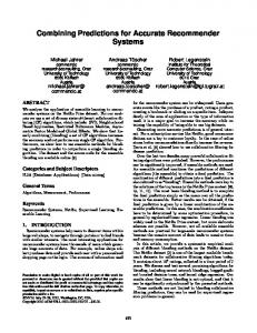
Figure 2: A push attack event stands out clearly when viewed through the lens of sample average and sample entropy. The window size is 50 and the window containing attacks is marked with a circle. anomaly by testing whether the absolute value of its z-score (the difference from the mean divided by the standard deviation) for sample average (sample entropy) is larger than a threshold. The threshold is set to 2 in this paper, which corresponds to the 95.5% confidence level. We illustrate the effectiveness of this approach through the example in Fig. 2. In this example, 40 attack ratings are injected to give the highest rating to a target item. The window size is 50 and the window containing attacks is marked with a circle. Both plots show that the attack event stands out clearly, while zscores for sample average and sample entropy of those windows containing normal ratings vary within a small range.
4. A THEORETICAL ANALYSIS Having introduced how to construct the time series for an item, we now quantify the changes of sample average and sample entropy caused by an attack event. Our discussion below is focused on a target item, and the notation used previously for Proposition 1 and 2 will still apply here. We note that the following analysis also holds for other items affected by attacks, e.g., filler items in segmented attacks. When attack ratings for the target item are injected, more than one window may contain attack ratings. We focus our analysis on the window that has the largest number of attack ratings, and denote it as the anomalous window. In case
there are two or more candidates for the anomalous window, one is chosen randomly. In the following, we will first compute the expected fraction of attack ratings in the anomalous window (Sec. 4.1); and then find the optimal window size k to maximize the absolute value of its z-scores for sample average (Sec. 4.2) and for sample entropy (Sec. 4.3). Maximizing the absolute value of these two z-scores helps to identify the anomalous window more accurately in our approach.
4.1
The expected fraction of attack ratings
Assuming that the number of attack profiles during an attack event is n, the number of attack ratings for the target item is also n. For ease of expression, we will initially assume that there are no normal (real) ratings given to the target item during the attack. In other words, the n attack ratings are consecutive. The more general situation in which real ratings and attack ratings are intermixed will be discussed in Sec. 4.4. Because the start position of attack ratings is random, we now compute the expected fraction (denoted as λ) of attack ratings in the anomalous window in each of the following three cases. In case 1 where n ≥ 2k − 1 (k ≤ dn/2e), there always exists a window that is filled with attack ratings. Therefore, we have λ = 1. In case 2 where dn/2e < k < n, we compute λ by moving a window (initial window in Fig. 3) from the start of attacks to the end of attacks. The right plot shows the number of attacks in the anomalous window when the initial window is in different positions. Overall, the expected number of attacks in the anomalous window is the area of the right plot divided by n, which gives us 2k − k 2 /n − n/4. Thus, λ in this case is 2 − k/n − n/(4k).
n a.
a.
0
attack ratings
0
initial window
k
�
previous window
c.
If the fraction of attack ratings in the anomalous window is λ0 , the entropy of w can be bounded using the following idea. To generate a rating in w, we first toss a coin. With probability 1 − λ0 , a normal rating is generated from the original distribution P ; and with probability λ0 , the highest rating rmax is generated. If the random variable that describes the outcome of the coin toss is denoted as C, we have, �
b.
n/2
previous window
b.
c.
n
0
n/2
n
Figure 4: The number of attacks in the anomalous window when the start position of the initial window moves from the start of attacks to the end of attacks in case 3 (k ≥ n). In case 3 where k ≥ n, λ can be computed in a similar way to the above. The expected number of attacks in the anomalous window is the area of the right plot in Fig. 4 divided by n, that is 3n/4. Thus, λ = (3n)/(4k). Combining all three cases, we conclude that the expected fraction of attack ratings in the anomalous window is
H(w) ≤ H(w, C) = H(C) + H(w|C) = H2 (λ0 ) + (1 − λ0 )H ≤ 1 + (1 − λ0 )H, �
�
0
0
�
1 2− 3n 4k
k n
n 4k
−
k ≤ dn/2e dn/2e < k < n k≥n
(1)
4.2 Sample average
�
�
�
E(M (w)) − µ √ σ/ k �
(3)
�
As λ = E(λ ), by Proposition 2 we have |E(ZH (w))| =
H − E(H(w)) √ , Var(− log2 p(x))/ k �
�
By Inequality (2, 3), |E(ZH (w))| can be bounded as √ √ k(λH − 1) kλH ≤ |E(ZH (w))| ≤ . (4) Var(− log2 p(x)) Var(− log2 p(x)) �
�
�
�
�
(2)
0
0
�
Denote the anomalous window as w, and denote its z-score for sample average as ZM (w). We now quantify the expectation of ZM (w) and compute the optimal k that maximizes its absolute value. Assuming w.l.o.g. that the item is being pushed, by Proposition 1 it follows that |E(ZM (w))| =
0
H(w) ≥ H(w|C) = (1 − λ0 )H.
�
�
0
where H2 (λ ) = −λ log2 λ − (1 − λ ) log2 (1 − λ ). On the other hand,
�
λ=
�
= =
(1 − λ)µ + λrmax − µ √ σ/ k √ kλ(rmax − µ) . σ
Using the same reasoning in Sec. 4.2, the upper bound of √ Inequality (4) is maximized when k = 2+6 7 n. Similarly, the √ 2H−1+ 7H 2 −4H+1 lower bound is maximized when k = n. 6H √ 2+ 7 Because this term converges to 6 n when H is large, we obtain the following theorem. Theorem 2. The absolute value of the expected z-score for sample entropy in the √ anomalous window, |E(ZH (w))|, is maximized when k ≈ 2+6 7 n (for large H). �
Since µ and σ are fixed, √ maximizing |E(ZM (w))| is reduced to maximizing the term kλ. Because λ has three different representations when k is changed (recall from Eq. 1), we do the optimization in each case. √ √ In case 1 where k ≤ dn/2e, λ = 1. Thus, we have kλ = k. This is maximized k = dn/2e. The maximum √ when √ value is dn/2e ≈ ( 2/2) n. In case 2 where dn/2e √ √