Attitudes and Value of Time Heterogeneity
Maya Abou-Zeid1, Moshe Ben-Akiva2, Michel Bierlaire3, Charisma Choudhury4, Stephane Hess5
Abstract There is ample evidence showing a high level of heterogeneity of values of time among travelers. Previous studies have represented this heterogeneity by a distribution such as lognormal whose parameters depend on covariates like income, trip purpose, and mode of travel. We present and demonstrate a model where the distribution of the value of time also depends on attitudes towards travel. Attitudes are latent, or unobservable, and their distribution determines the conditional distribution of the value of time given the observable covariates such as income. We illustrate this model using data from a stated preferences survey. The estimation results show that as expected the median value of time increases with income and that the variability of value of time also increases with income reflecting the greater effect that the attitude towards travel has for high income groups.
1
American University of Beirut, Department of Civil and Environmental Engineering. Phone: +961-1-350000 Ext. 3431. Fax: +961-1-744462. E-mail:
[email protected]. 2 Massachusetts Institute of Technology, Department of Civil and Environmental Engineering. Phone: +1-617253-5324. Fax: +1-617-253-0082. E-mail:
[email protected]. 3 Ecole Polytechnique Fédérale de Lausanne, Transport and Mobility Laboratory, School of Architecture, Civil and Environmental Engineering. Phone: +41-21-693-25-37. Fax: +41-21-693-80-60. E-mail:
[email protected]. 4 Bangladesh University of Engineering and Technology, Department of Civil Engineering. Phone: +88-029665650 Ext. 7201. Fax: +88-02-8613026. E-mail:
[email protected]. 5 University of Leeds, Institute for Transport Studies. Phone: +44-0-113-34-36611. Fax: +44-0-113-343-5334. E-mail:
[email protected].
1
1. Introduction The concept of valuation of travel time is based on the fact that time is considered as a resource, which is clearly limited and, consequently, has a value. The willingness to pay by an individual to save one unit of travel time in is the value of travel time savings. More generally the trade-off between travel time and travel cost in individuals‟ evaluation of travel alternatives is referred to as the value of travel time (VOT). It plays an important role in costbenefit analysis of public sector investments in transportation. Recognition of the value of the time dimension of travel can be traced back to Jules Dupuit (1844, 1849), a French inspector of bridges and highways who is considered to be the pioneer of transportation economics. A more recent treatment of the value of time is given by Train and McFadden (1978) who consider its effect on the choice of travel mode in the context of the trade-off between the consumption of goods and leisure. Empirical measurement of VOT is obtained by calculating a traveler‟s sensitivity to time relative to cost (see, for example, the transportation economics textbook by Blauwens et al., 2008). VOT varies across travel situations and individuals. It may depend on the enjoyment of travel, the use of the travel time to conduct other activities, the comfort and reliability of the mode, the time pressure, and the affordability of the travel cost. These factors cause people to develop attitudes towards travel modes that in turn affect their VOT. Typically, the empirical estimation of VOT accounts for the effects of these attitudes by modeling the VOT as a function of trip purpose, time-of-day, income, and other socioeconomic and demographic characteristics such as occupation, employment status, age, and gender. It has been shown in previous studies that these types of variables do not fully account for the heterogeneity in the VOT and therefore it is represented by a distribution such as log-normal whose parameters depend on these covariates (see, for example, Ben-Akiva et al., 1993). The state-of-the-art approach to capture this distribution is to use a logit mixture 2
model where the mixing distribution represents the distribution of the travel time and cost parameters (e.g. Algers et al., 1998, Hess and Axhausen, 2004, and Fosgerau, 2005). The large coefficients of variation of the distributed values of time obtained in these logit mixture estimations indicate that there is scope for improving the VOT estimates by capturing the unobserved heterogeneity in a more systematic manner. The purpose of this paper is to show that this variability may be explainable by individuals‟ attitudes towards travel. An example would be an individual‟s degree of like or dislike for travel by a particular mode such as a „car-loving‟ attitude held by an individual who believes that public transportation is uncomfortable or unreliable. A traveler with such attitude is likely to be more sensitive to the time and cost changes associated with public transportation trips compared to another traveler who has a positive attitude towards public transportation (e.g. perceiving it as more environment-friendly, sustainable, and/or convenient). The VOT associated with public transportation will consequently be different for the two travelers. In this paper we extend the logit mixture approach to capture the effects of attitudes and perceptions on the time and/or cost sensitivities using structural and measurement equations in addition to a choice model. We use this extended framework to demonstrate the effects of attitudes on VOT through a case study. Though there has been quite a substantial research on capturing the effects of attitudes and perceptions in a mode choice context (e.g. Koppelman and Hauser, 1978, Proussaloglou, 1989, Golob and Hensher, 1998, Golob, 2001, Outwater et al., 2003, and Johansson et al., 2006), to our knowledge, this is the first research that explores their effects on VOT. The rest of the paper is organized as follows: an overview of discrete choice models with latent constructs is presented first. The model formulation is presented next. This is followed by a case study using stated preferences (SP) data. The results are summarized and the paper concludes with directions for future research.
3
2. Discrete Choice Models with Latent Constructs As mentioned above, the importance of attitudes and perceptions in explaining choice behavior has been acknowledged for a long time. More recently, the Hybrid Choice Model (HCM) has been proposed by Ben-Akiva et al. (2002 a and b), Morikawa et al. (2002), and Walker and Ben-Akiva (2002) as a framework including latent variables and latent classes, where psychometric indicators are combined with choice data to estimate the model. The framework is depicted in Figure 1, where the following conventions are used. Observed quantities, such as explanatory variables, as well as choices and psychometric indicators, are represented in rectangular boxes. Latent constructs, such as utilities, latent classes, and latent variables, are represented in ovals. Solid arrows represent a causal link between two constructs. Dashed arrows represent measurements, while dotted arrows represent the contribution of error terms capturing various types of uncertainty.
Explanatory Variables
Errors
Errors
Psychometric Indicators
Latent Classes
Latent Variables
Psychometric Indicators
Errors Utility
Stated Choice
Revealed Choice
Figure 1: Hybrid Choice Model (Walker and Ben-Akiva, 2002)
The conventional discrete choice model is actually a specific instance of this framework, as depicted in Figure 2. 4
Explanatory Variables
Errors Utility
Choice
Figure 2: The conventional discrete choice model
The concept of utility is latent. The causal relationship between the explanatory variables and the utility is captured by a structural equation such as the following: U
V X,
(1)
where U is a vector of utilities of all alternatives, V is a vector of systematic utilities that is a function of explanatory variables X and parameters , and is a vector of error terms. A measurement equation links the latent utility with an observable quantity. For the random utility model, the choice indicator of alternative i is expressed as follows:
yi
1
if U i
Uj
0
otherwise
j
i
, i 1, , J
(2)
where yi is a choice indicator that is equal to 1 if alternative i is chosen and is 0 otherwise, Ui denotes the utility of alternative i, and J is the number of alternatives. The HCM combines a choice model with a latent variable model. The latent variable model adds behavioral richness as it can be used to model the formation of latent (unobserved) psychological constructs such as attitudes, perceptions, and plans and, through its linkage to the choice model, allows a representation of the effect of these constructs on preferences. The evolution of psychological constructs can also be accommodated within a dynamic version of
5
the HCM which combines a Hidden Markov model with a discrete choice model (Ben-Akiva et al. 2006, Choudhury et al. 2007, Ben-Akiva, 2010).
3. Model Formulation The general model framework proposed in this research is an application of the Hybrid Choice Model discussed in the previous section and can be represented by Figure 3. The utilities are functions of attributes of the alternatives (time, cost, etc.) obtained from revealed or stated preferences data (RP or SP), characteristics of the traveler (income, age, etc.), and his/her attitudes towards the alternative modes (pro-car, pro-public transportation, etc.). The sensitivity to attributes, including time and cost, can vary with the attitudes towards the alternatives. The attitudes in turn depend on the characteristics of the traveler as well as his/her current experience with the alternative used in the RP case. The attitudes are unobserved and are measured by indicators (such as responses to attitudinal questions). The utility is measured by the choice indicator.
6
Figure 3: General model framework
The specifications of the utility equations (3) and the equations capturing the relationships between the attitudes and the RP attributes and socio-economic characteristics (4) constitute the structural model whereas the choice indicator equations (5) and the relationships among the attitudes and the observed indicators (6) constitute the measurement model, as follows: Structural Model U
X1
A
X2
X1 A
(3) (4)
where U is a vector of utilities of all alternatives, X1 and X2 are matrices of explanatory variables, A is a vector of attitudes, parameters, and and
and
are vectors of parameters,
are vectors of error terms.
7
is a matrix of
Measurement Model
yi I
1
if U i
Uj
0
otherwise
j
i
, i 1, , J
(5)
(6)
A
where I is a vector of attitudinal indicators,
is a matrix of parameters,
is a vector of error
terms, and the remaining terms are as previously defined. The likelihood function for a given observation is the joint probability of observing the choice and the attitudinal indicators as follows:
f y, I X
P y X , A f I I A f A A X dA
(7)
A
where y is a vector of choice indicators, the conditional distribution P y X , A of y given X and A is obtained from Equations (3) and (5) and an assumed distribution of , the conditional density f I I A of I given A is obtained from Equation (6) and an assumed distribution of , and the density f A A X of A given X is obtained from Equation (4) and an assumed distribution of
. The dimensionality of the integral in (7) is equal to the number of latent
attitudes.
4. Case Study In this section, we present a case study to illustrate the effect of attitudes on value of time. The case study is based on data from a stated preferences (SP) survey conducted in Stockholm, Sweden, in 2005 among 2400 households consisting of married couples where both husband and wife are working or studying (Transek, 2006). The SP choice scenarios included choices between car and public transportation as well as choices between car options (which differed in terms of travel times, costs, and number of speed cameras along the route). Responses from within-mode car experiments have been used in this study. 8
4.1 Data The sample used for estimation consists of 2216 SP responses from 554 individuals. In the survey, each respondent was presented with four SP scenarios involving choice between two car alternatives (which differed in terms of travel times, travel costs, and number of speed cameras along the route). The respondents also had the option to choose „Indifferent‟. The data cover people from various income groups, the average monthly individual income being around 31,500 Swedish Kronas (around 4000 USD). 55% of the respondents are female. The attitudinal questions presented to the respondents are shown in Table 1. In each case, the respondents were asked to indicate to what extent they would agree with a specific statement on a 5-point scale (where 1 is “Do not agree at all” and 5 is “Do fully agree”). “No experience” was also an option. Table 1: Attitudinal questions 1
It is comfortable to go by public transportation to work.
2
It feels safe to go by public transportation.
3
Going by public transportation is worth its price compared to going by car.
4
It is comfortable to go by car to work.
5
It feels safe to go by car.
6 7
The one in the household that needs the car most for the work trip is the one that uses the car. In our family we are equals when deciding who is going to use the car.
8
We share household work equally in our household.
9
Women drive safer than men.
10
It is very important that traffic speed limits are not violated.
11
I am positive towards increased speed monitoring by cameras.
12
Increase the motorway speed limit to 140 km/h.
13
The 30 km/h speed limit in dwelling areas is needed.
14
Measures to improve public transportation should be undertaken.
15
I consciously limit my car use to reduce emissions.
Among these, perceptions/attitudes regarding comfort, safety, adherence to speed limits, and increase of speed limits to 140 km/hr (questions 4, 5, 10 and 12) are the ones that
9
are most likely to reflect the car-loving attitude and are expected to have the most significant impacts on the sensitivity to time and cost associated with the car alternatives. We have selected these indicators in the model specification described in Section 4.2. As another example, attitudinal statements related to the presence of speed cameras and reduction of speed limit in residential areas (questions 11 and 13) are likely to reflect an attitude towards speed and safety. As this attitude is less directly related with value of time, this latent variable is not included in the model described in Section 4.2. The summary of the responses to these key indicators is listed in Table 2. Table 2: Summary of responses to the key attitudinal questions Measure Car comfortable Car safe Important not to violate speed limits Positive towards speed cameras Increase speed limit on highway to 140 km/h Decrease in speed limit in residential areas to 30 km/h
1 4% 2% 6% 27% 12% 5%
2 6% 6% 23% 15% 6% 3%
3 9% 15% 29% 24% 9% 11%
4 20% 30% 22% 16% 20% 17%
5 61% 47% 21% 17% 53% 63%
Average 4.3 4.1 3.3 2.8 3.9 4.23
As seen in Table 2, most of the indicators (except the one regarding decrease in speed limit in residential areas) indicate a positive attitude towards car. However, the need for decrease in speed limit in residential areas may be confounded with non-travel related attitudes as well (e.g. desire for a safer residential neighborhood) and was not included in the model.
4.2 Specification of Latent Attitude Model A simplified version of the general model was formulated for this application since no revealed preferences (RP) data were available (Figure 4). The attitudes were therefore assumed to be functions of socio-economic and demographic variables only. Also, because the choice is between car alternatives, a single attitude - positive attitude towards car - was included in the model (referred as „car-lover‟ in the subsequent sections).
10
Figure 4: Model structure
The structural model in this case therefore includes the specification of the utility equations of the alternatives and the relationship between attitude and socio-economic variables. The measurement equations capture the relationships between the indicators and the „car-lover‟ attitude as well as the relationship between the utilities and the final choices. Each model component is described below.
4.2.1 Structural Model Utility Equations The utility of each of the car alternatives (denoted as „Car 1‟ and „Car 2‟ in the equations below) is a function of attributes of the alternative (time, cost, and number of speed cameras), socio-economic characteristics of the traveler (through the interaction of income with cost), and the traveler‟s attitude towards the car interacted with cost/income. The systematic utility of the „Indifferent‟ alternative (denoted as „Indifferent‟ in the equations
11
below) is normalized to zero. The resulting utilities can be expressed by the following equations: U Car 1
1
Time
Time Car 1
Cost
Camera Car 1
Car 1
Time Car 2
Cost
Camera
U Car 2
2
Time
Camera Car 2
Camera
U Indifferent
Cost Car 1 Income
0
Cost Car 1 Income
Cost Car 2 Income
Cost Car 2 Income
Attitude Car
Attitude Car
(8)
(9)
Car 2
(10)
Indifferent
where: TimeCar 1, TimeCar
2
= travel time associated with car alternatives 1 and 2, respectively
(minutes); CostCar 1, CostCar 2 = travel cost associated with car alternatives 1 and 2, respectively (Swedish Kronas); CameraCar 1, CameraCar 2 = number of speed cameras associated with car alternatives 1 and 2, respectively; AttitudeCar = attitude towards the car (a higher value indicates a more positive attitude towards the car); Income = monthly individual income (1000‟s of Swedish Kronas); 1
,
Car1
2
,
,
Time
Car 2
,
,
,
Cost
Indifferent
Camera
, = parameters;
= random error terms, i.i.d. EV(0,1).
Attitude Equation The attitude is modeled as a function of socio-economic and demographic characteristics (observed) and can be expressed as follows: Attitude Car
0
Female
Female
Age
Age 1
Educ 1
Educ 1
55
Income
Income Age 2
Educ 2
Age 55 - 65
Educ 2
Educ 3
12
Age 3
Educ 3
Age Car
65
(11)
where: Female = female dummy variable, 1 if female, 0 otherwise; Income = monthly individual income (10,000‟s of Swedish Kronas); Age < 55, Age 55-65, and Age > 65 = different age ranges used in a piecewise linear specification of age defined by breakpoints at the ages of 55 and 65; Educ 1, Educ 2, Educ 3 = education dummy variables: Educ 1 = 1 if respondent has basic schooling / pre-high school education, 0 otherwise; Educ 2 = 1 if respondent has university education, 0 otherwise; Educ 3 = 1 if respondent has other education, 0 otherwise (the base education category is high school); 0
,
Female
,
Income
,
Age 1
,
Age 2
,
Age 3
,
Educ 1
,
Educ 2
,
Educ 3
,
Car
= parameters;
= random error term, N(0,1).
4.2.2 Measurement Model Choice Model The choice between the alternatives is assumed to be based on utility maximization and can be expressed as follows:
yi
1 if U i
Uj j
0 otherwise
i
, i = Car 1, Car 2, Indifferent
(12)
where yi is a choice indicator, 1 if alternative i is chosen, 0 otherwise. Attitudinal Measures Four measures are used as indicators of the „car-lover‟ attitude as shown in Equations (13)-(16). The first equation is normalized by setting the intercept term to 0 and the coefficient of attitude to 1. The indicators are specified as continuous variables for simplicity.
I1
1
I2
2
Attitude Car
1
2
Attitude Car
1
;
1
0,
1
(13)
1
(14)
2
13
Attitude Car
3
(15)
Attitude Car
4
(16)
I3
3
3
I4
4
4
where:
I1, I 2 , I3 , I 4 = responses to attitudinal questions ( I1 = “car safe”; I 2 = “car comfortable”; I3 = “important not to violate speed limits”; I 4 = “increase speed limit on highway to 140 km/h); 1
, 2 , 3,
4
1
~ N 0,
,
2
,
3
= random error terms:
4
,
2
~ N 0,
2
,
1
2
~ N 0,
2 2
,
3
~ N 0,
2 3
,
;
4
4
1
, 1,
2
,
3
,
4
,
1
,
2
,
3
,
4
= parameters.
4.2.3 Likelihood Function The maximum likelihood method is used for model estimation. The likelihood of a given observation is the joint probability of observing the choice and the four indicators of the attitude „car-lover‟. Conditional on the attitude (and consequently on
, the error term in
the attitude structural equation), the choice probability and the four indicator density functions are independent. Therefore, the likelihood is obtained by integrating the product of the conditional probabilities (of the choice and indicators) over the distribution of
as shown
in Equation (17). f y, I X
P y X,
f1 I1
f2 I2
f3 I3
f4 I4
f5
d
…………………………..(17)
where:
P y X,
fk Ik
is a logit model.
Ik
1 k
k
k
Attitude Car
, k 1,2,3,4
k
14
(18)
(19)
f5 and
is the standard normal density function.
4.3 Specification of Base Model (without Latent Attitude) For comparison purposes, a base model that does not include latent attitudes was estimated as will be discussed in the next section. The structural equations of the base model consist of the utility equations (20-22) (specified as in the latent attitude model but excluding the attitude variable). The measurement equation consists of the choice model as shown in Equation (23).
UCar1
1
UCar 2
2
U Indifferent yi
Time
Time Car1
Time
0
1 if U i
Time Car 2
Cost
CostCar1 Income
Cost
CostCar 2 Income
CameraCar1
Camera
0 otherwise
Car 2
(20) (21) (22)
Indifferent
Uj j
CameraCar 2
Camera
Car1
i
, i = Car 1, Car 2, Indifferent
(23)
The likelihood function for a given observation is the choice probability P y X which is given by the logit model.
4.4 Results 4.4.1 Estimation Results for Base model The model was estimated using the latest version of BIOGEME (Bierlaire and Fetiarison, 2009). The estimation results for the base model are summarized in Table 3. We see the expected negative marginal utilities for travel time and travel cost, along with a negative effect associated with increases in the number of speed cameras. Additionally, we obtain positive estimates for the two alternative specific constants (ASCs). This is the result 15
of the low rate of choice for the Indifferent option, while the larger value of the first ASC can be explained by a mixture of inertia effects (first alternative is a status quo option) and reading left to right effects. Table 3: Estimation results for base model (N = 2216 observations; total log-likelihood = -1575.566) Parameter / Variable
Estimate
Robust Std error
Robust t-statistic
1
4.03
0.257
15.68
2
2.86
0.268
10.68
Time
-0.0397
0.00482
-8.23
Cost / Income
-0.953
0.191
-4.98
Number of speed cameras
-0.110
0.0396
-2.78
4.4.2. Estimation Results for Latent Attitude Model The estimation results for the latent attitude model are summarized in Table 4. The following analysis considers the results in two stages, namely the structural model and the measurement model.
16
Table 4: Estimation results for latent attitude model (N = 2216 observations; total log-likelihood = -15,266.435) Parameter / Variable
Estimate
Robust Std error
Robust t-statistic
1
4.01
0.258
15.58
2
2.84
0.269
10.57
-0.0388
0.00479
-8.10
-2.02
0.557
-3.63
0.265
0.126
2.11
-0.109
0.0397
-2.75
5.25
0.584
8.99
-0.0185
0.0545
-0.34
Income
0.0347
0.0174
1.99
Age < 55
-0.0217
0.0118
-1.85
Age 55-65
0.00797
0.00909
0.88
Age > 65
0.0231
0.00986
2.35
Education: primary
-0.147
0.156
-0.94
Education: university
-0.252
0.0483
-5.22
Education: other
-0.157
0.184
-0.85
0.934
0.0577
16.18
1
0
-
-
2
1.13
0.385
2.93
3
3.53
0.186
19.02
4
1.94
0.301
6.45
1
1
-
-
2
0.764
0.0933
8.19
3
-0.0716
0.0441
-1.62
4
0.481
0.0720
6.68
1
0.566
0.0927
6.10
2
0.909
0.0375
24.26
3
1.25
0.0156
79.71
4
1.37
0.0226
60.73
Structural Model Utility
Time Cost / Income Cost / Income
AttitudeCar
Number of speed cameras Attitude 0
Female
Car
Measurement Model
Structural Model Just as for the base model, the signs of the travel time, travel cost, and speed camera coefficients are as expected; the findings for the ASCs are also in line with those obtained for
17
the base model. As to the role that the latent attitude plays in the cost sensitivity, the positive estimate shows that with an increasing value for the latent attitude, the cost sensitivity is lower. Moreover, the attitude variable is significant at the 95% level of confidence. The latent variable was specified with a view to capturing the attitude towards car, and an increasingly positive attitude has a reducing effect on the cost sensitivity for car travel. In terms of the effects of socio-economic and demographic variables on the latent attitude, the effect of gender is insignificant, while increasing income leads to an increasingly positive attitude towards car. For the lowest age group, i.e. respondents aged between 42 and 55 (there were no respondents in the dataset with age less than 42), there is a small gradual reduction in the positive attitude towards car with increasing age. In the category for respondents aged between 55 and 65, the change across different ages is not significant, while, for respondents aged above 65, there is an increasing positive impact on the latent attitude with increasing age. Finally, in terms of education, with high school education serving as the base, we note that there are no significant differences in the latent attitude for respondents with primary (basic schooling / pre-high school) education only or for respondents with other types of education, while on the other hand, there is evidence of a negative effect on the latent attitude if respondents have a university degree. Measurement Model The attitude is used as an explanatory variable for the four indicators, with the coefficient of attitude in the car comfortable indicator equation being normalized to 1. Here, we can see that an increasingly positive attitude to car will lead to respondents being more in agreement with statements in relation to car safety as well as increasing speed limit on the highway. On the other hand, they are less likely to agree with the statement that it is important not to violate speed limits, but the associated coefficient is very small and only significant at the 90% level. 18
4.4.3 Analysis of VOT Findings In this section, we analyze the implied value of time (VOT) resulting from our models. In the base model, the cost sensitivity was a function of the respondent‟s income, leading to a distribution of the VOT across the seven distinct income groups in our sample population. In the latent attitude model, the cost sensitivity was additionally a function of the latent attitude, where this in turn was a function of gender, income, age, and level of education, as discussed above. The following analysis considers both the VOT distribution across the entire sample and the VOT distribution within each of the seven income groups. For the latter, a point value will be obtained with the base model (given that income was the only interaction), while, in the latent attitude model, we obtain further heterogeneity within these subsegments of the sample population. In the base model, the VOT only depends on income and can be expressed as follows:
VOT
Time
(24)
Income
Cost
Therefore, we obtain a single VOT for each respondent that depends on income. For the latent attitude model, the VOT depends on income and attitude and can be expressed as follows:
Time
VOT Cost
Attitude Car
Income
(25)
The attitude is a latent variable that has a random disturbance, as given in Equation (11), and therefore the attitude is distributed. From the relationship between the VOT and income and attitude (Equation 25) and the distribution of the attitude (based on Equation 11), we derive the distribution of VOT conditional on income and the explanatory variables determining the 19
attitude. By integrating it over the sample distribution of the explanatory variables determining the attitude, we obtain the distribution of the VOT conditional on income. While in the base model a given income produces a single VOT, in the latent attitude model a given income is associated with a distribution of VOT. In the following analysis, the calculation of this conditional distribution of VOT is done by simulating multiple draws from the distribution of the disturbance of the attitude for every individual and then empirically using these draws to generate a distribution of VOT for a given income group. Given the use of a Normal distribution for the random disturbance in the latent attitude, the moments of the VOT distribution in this model are not defined (see, for example, Daly et al., 2010). Nevertheless, it remains common practice to use simulation of this ratio to produce „estimates‟ for these moments. However, recent results by Daly et al. (2010) show that this can mask the issue, where, with model specifications that imply infinite moments, the use of simulation of the ratio involving a randomly distributed cost coefficient can produce results that imply finite moments. Additionally, the results are highly dependent on the draws used in simulation, with results in the work by Daly et al. showing that even when making use of 10,000,000 draws, simulation runs with different sets of draws show great variation in the results for the simulated moments. For this reason, our presentation relies on various percentiles (10%, 25%, 50%, 75%, 90%) as shown in Table 5 as well as a graphical representation of the VOT distribution as shown in Figure 5, where the above work shows that these percentile measures always exist and that they are stable across different simulation runs. The results are shown for the entire sample as well as for the seven distinct income groups. For the base model, we show the minimum, median, mean, and maximum VOT in the overall sample, along with the single values for each of the seven income segments. For
20
the latent attitude model, we show the above mentioned percentile points, along with the difference between the 90th percentile and the 10th percentile. The results show consistency between the median values in the seven separate income groups and the corresponding point values from the base model. For the overall sample, the median from the latent attitude model is roughly halfway between the median and mean from the base model, while, for the separate income classes, the point value from the base model always corresponds closely to the median from the latent attitude model. The upper tail of the sample level distribution has more weight in the latent attitude model than in the base model, which is to be expected, and the absolute level of heterogeneity increases with income, while the relative degree of variation (when taking into account the change in median) is quite stable across the seven income groups. Table 5: VOT findings Base model VOT (SEK/hr)
Latent attitude model VOT (SEK/hr)
Respondents
Min
median
Mean
max
10%
25%
median 75%
Full sample
554
28.12
68.74
78.90
149.97
40.89
53.62
73.70
104.56 145.37 104.48
Income group 1
23
28.12
20.42
23.22
27.33
33.18
41.10
20.68
Income group 2
58
43.74
32.49
36.98
43.75
53.33
66.97
34.48
Income group 3
127
56.24
41.57
47.22
55.76
67.97
84.30
42.73
Income group 4
97
68.74
50.67
57.62
67.93
82.86
103.03 52.36
Income group 5
137
87.48
64.69
73.45
86.63
105.50 131.51 66.82
Income group 6
55
112.48
83.89
95.48
112.89
137.74 172.14 88.25
Income group 7
57
149.97
112.16 127.77 150.79
21
90%
90%-10%
184.50 230.68 118.52
Figure 5: VOT distribution
22
5. Conclusion Previous studies have applied logit mixture models to estimate distributions of value of time conditional on income and other covariates. In this paper, we have extended that approach by using a behavioral approach to specify the mixing distribution. The approach entails the specification of a latent variable model that quantifies the attitudes that affect the value of time. We illustrated the idea through a stated preferences study of choice between two car alternatives that differ on travel time, travel cost, and number of speed cameras along the route. We developed a Hybrid Choice model that incorporates a latent „car-loving‟ attitude as an explanatory variable influencing the cost sensitivity of travelers. The estimation results show that as expected the median value of time increases with income and that the variability of value of time also increases with income reflecting the greater effect that the attitude towards travel has for high income groups. The limitations of the available data precluded the possibility of a more elaborate attitudinal model. In further research, the approach should be extended to allow for multiple attitudes to separately capture those attitudes that affect time sensitivity and others that affect cost sensitivity.
23
References 1. Algers, S., Bergström, P., Dahlberg, M., and Lindqvist Dillén, J. (1998) “Mixed Logit estimation of the value of travel time”, Working Paper Series 1998:15, Uppsala University, Department of Economics. 2. Ben-Akiva, M. (2010) “Planning and action in a model of choice”, in Choice Modelling: The State-of-the-Art and the State-of-Practice: Proceedings from the Inaugural International Choice Modelling Conference, S. Hess and A. Daly (eds.), Emerald, 19-34. 3. Ben-Akiva, M., Bolduc, D., and Bradley, M. (1993) “Estimation of travel choice models with randomly distributed value of time”, Transportation Research Record, 1413, 88-97. 4. Ben-Akiva, M., Choudhury, C. F., and Toledo, T. (2006) “Modeling latent choices: application to driving behavior”, Paper presented at the 11th International Conference on Travel Behaviour Research, Kyoto, Japan. 5. Ben-Akiva, M., McFadden, D., Train, K., Walker, J., Bhat, C., Bierlaire, M., Bolduc, D., Boersch-Supan, A., Brownstone, D., Bunch, D. S., Daly, A., de Palma, A., Gopinath, D., Karlstrom, A., and Munizaga, M. A. (2002a) “Hybrid Choice Models: progress and challenges”, Marketing Letters, 13(3),163-175. 6. Ben-Akiva, M., Walker, J., Bernardino, A., Gopinath, D., Morikawa, T., and Polydoropoulou, A. (2002b) “Integration of Choice and Latent Variable Models”, in Perpetual Motion: Travel Behaviour Research Opportunities and Application Challenges, H. Mahmassani (ed.), Elsevier Science, 431-470.
24
7. Bierlaire, M. and Fetiarison, M. (2009) “Estimation of discrete choice models: extending BIOGEME”, Proceedings of the 9th Swiss Transport Research Conference (STRC), September 9 - 11, 2009. 8. Blauwens, G., De Baere, P., and Van de Voorde, E. (2008) Transport Economics, Third Edition, Uitgeverij De Boeck. 9. Choudhury C., Toledo, T., Rao, A., Lee, G., and Ben-Akiva, M. (2007) “State dependence in lane changing models”, in Transportation and Traffic Theory, R. Allsop, M. G. H. Bell, and B. G. Heydecker (eds.), Elsevier, 711-733. 10. Daly, A. J., Hess, S., and Train, K. E. (2010) “Ensuring finite moments for willingness to pay in random coefficients models”, ITS working paper. 11. Dupuit, J. (1844) “On the measurement of the utility of public works”, Annales des Ponts et Chaussées. (English translation, International Economic Papers, 1952, 2, 83-110). 12. Dupuit, J. (1849) “On tolls and transport charges”, Annales des Ponts et Chaussées. (English translation, International Economic Papers, 1962, Vol. 11, pp. 7-31). 13. Fosgerau, M. (2005) “Unit income elasticity of the value of travel time savings”, NECTAR Conference, Las Palmas G.C., 2005. 14. Golob, T. (2001) “Joint models of attitudes and behavior in evaluation of the San Diego I-15 congestion pricing project”, Transportation Research Part A, 35,495514.
25
15. Golob, T. and Hensher, D. (1998) “Greenhouse gas emissions and Australian commuters‟ attitudes and behavior concerning abatement policies and personal involvement”, Transportation Research Part D, 3, 1-18. 16. Hess, S. and Axhausen, K. (2004) “Checking our assumptions in value-of-traveltime modelling: Recovering taste distributions”, CTS Working Paper, Centre for Transport Studies, Imperial College London. 17. Johansson, V., Heldt, M. and Johansson, P. (2006) “The effects of attitudes and personality traits on mode choice”, Transportation Research Part A, 40(6), 507525. 18. Koppelman, F. S. and Hauser, J. R. (1978) “Destination choice behavior for nongrocery shopping trips”, Transportation Research Record, 673, 157-165. 19. Morikawa, T., Ben-Akiva, M., and McFadden, D. (2002) “Discrete choice models incorporating revealed preferences and psychometric data”, Econometric Models in Marketing, Advances in Econometrics, 16, P. H. Franses and A. L. Montgomery (eds.), Elsevier, 29-55. 20. Outwater, M. L., Castleberry, S., Shiftan, Y., Ben-Akiva, M., Zhou, Y., and Kuppam, A. (2003) “Use of structural equation modeling for an attitudinal market segmentation approach to mode choice and ridership forecasting”, Paper presented at the Transportation Research Board Annual Meeting, Washington DC. 21. Proussaloglou, K. (1989) “Use of travelers‟ attitudes in rail service design”, Transportation Research Record, 1221, 42-50. 22. Train, K. and McFadden, D. (1978) “The goods-leisure tradeoff and disaggregate work trip mode choice models”, Transportation Research, 12, 349-353.
26
23. Transek (2006) “Gender equity and mode choice”, Transek report 2006:22. 24. Walker, J. and Ben-Akiva, M. (2002) “Generalized random utility model”, Mathematical Social Sciences, 43(3), 303-343.
27