Autoassociative memory implemented with attractor neural networks works ..... It should be noted that although the system has never seen the noise free .... Hertz, J., A. Krogh, and R.G. Palmer, Introduction to the Theory of Neural Computation.
Attractor Memory with Self-organizing Input Christopher Johansson and Anders Lansner Department of Numerical Analysis and Computer Science, Royal Institute of Technology, 100 44 Stockholm, Sweden Fax: +46-8-7900930 {cjo, ala}@nada.kth.se
Abstract. We propose a neural network based autoassociative memory system for unsupervised learning. This system is intended to be an example of how a general information processing architecture, similar to that of neocortex, could be organized. The neural network has its units arranged into two separate groups called populations, one input and one hidden population. The units in the input population form receptive fields that sparsely projects onto the units of the hidden population. Competitive learning is used to train these forward projections. The hidden population implements an attractor memory. A back projection from the hidden to the input population is trained with a Hebbian learning rule. This system is capable of processing correlated and densely coded patterns, which regular attractor neural networks are very poor at. The system shows good performance on a number of typical attractor neural network tasks such as pattern completion, noise reduction, and prototype extraction.
1 Introduction Autoassociative memory implemented with attractor neural networks works best with sparse activity, i.e. when each stored pattern only activates a small fraction of the network’s units [1]. Further, this type of memory achieve a higher storage capacity with uncorrelated or weakly correlated, e.g. random, patterns than with highly correlated patterns. Real world data, e.g. sensor data, often consists of a large number of correlated measurements, resulting in densely coded and correlated input patterns. It has been suggested that for successful use of such raw data, the redundancies embedded in the data must be reduced and that this is done by the early sensory processing circuits, e.g. the primary visual cortex V1, in the mammalian brain [2]. At the same time as the redundancies in the sensory data are reduced, it is important to preserve the information in this data [3-6]. Linsker called this the Infomax principle. One way of assuring that the information present in the sensory data is maintained is to measure the reconstruction error of this data. Barlow argues, based on arguments of computational efficiency, that preprocessing of sensory data should generate a factorial code, i.e. a code that can represent the input data by a limited number of components. Further, this factorial code should be sparse. A sparse activity is also supported by arguments of neural energy efficiency [7, 8]. Algorithms that generates such sparse codes from real world image data have been explored by several authors [7-13]. A cause commonly mentioned by these A.J. Ijspeert et al. (Eds.): BioADIT 2005, LNCS 3853, pp. 265 – 280, 2006. © Springer-Verlag Berlin Heidelberg 2006
266
C. Johansson and A. Lansner
investigators for recoding the sensory information with a sparse code is that it is better suited for use in an associative memory, which is demonstrated in several papers [14-17]. By extracting features from the input data a sparse and information preserving recoding is achieved. A powerful and commonly used approach to feature extraction is to use multiple layers of hierarchically arranged feed-forward networks that implements competitive learning [3-6, 18-25]. This type of structures can achieve accurate and invariant pattern recognition, e.g. with slow learning [21]. In this paper we investigate an attractor neural network that is paired with a selforganizing and competitive learning input network. The resulting system can by unsupervised learning store densely coded and correlated patterns, e.g. the images in Fig. 1. The purpose of the input network is to reduce redundancies and sparsify the input data, which is achieved by means of competitive learning [26]. An important aspect of the proposed system is that it is implemented with biologically plausible learning rules. These are learning rules that are local in at least space, i.e. weight updates that only depend on variables present in the pre- and postsynaptic junction. To this class of learning rules we count Hebbian and competitive learning. This type of local algorithms has the advantage that they parallelize well on cluster computers and in general are very fast. Currently, few that work with biological models of the visual pathways have constructed larger systems that are capable of doing more than one step in the processing. Often, only a single specific component of the visual processing pathway is studied and modeled. A reason for this is that it is hard to get different models and neural network architectures to work properly together. One of the more interesting works that combines attractor neural networks with competitive learning is that by Bartlett and Sejnowski [16] who have built a neural system for viewpoint invariant face recognition. Here, we are not interested of building a system that can solve a particular task, although we use a selected problem for demonstration, but rather to build a general information processing system much like the brain like systems
Fig. 1. The data set has 36 patterns representing both letters and digits that were derived from the font Arial. Each pattern is shown as a black and white 16×16-pixel image.
Attractor Memory with Self-organizing Input
267
discussed by Hawkins [27]. We believe that attractor dynamics and distributed processing are important features of such system. The system that we propose in this paper can be used as a module in a larger hierarchal system, which is discussed in the end of this paper. The experiments in this paper use the data set shown in Fig. 1. It consists of 36 black and white images of letters and digits, each represented by 16×16 pixels. These images were derived from the Arial font, and on average they have as many black as white pixels. Although the proposed system is evaluated on tasks involving image data, it should not be compared to state of the art image processing algorithms [28, 29] because it is not intended for image processing in particular. The paper is organized as follows: In section 1.1 and 1.2 the learning rules, implemented in the system, are presented. In section 1.3, results on using the data set together with standard attractor neural networks is presented. In section 2, our system is described. In section 3 the results on applying the system to the image data are given. Section 4 contains a discussion of the results and future developments of the system. The conclusions are presented in section 5. 1.1 Bcpnn In the following we present the Bayesian Confidence Propagating Neural Network (BCPNN) with hypercolumns [30, 32]. This type of neural network can be used to implement both feed-forward classifiers and attractor memory. It has a Hebbian type of learning-rule, which means that it is local in both space and time (only the pre- and postsynaptic units activations’ at one particular moment are needed to update the weights) and therefore it can be efficiently parallelized. Further, the network can be used with both unary-coded activity (spiking activity), o∈{0,1}, and real-valued activity, o∈(0,1). The network has N units grouped into H hypercolumns with Uh units in each. Here, h is the index of a particular hypercolumn and Qh is the set of all units belonging to hypercolumn h. When an attractor network is implemented, a symmetric weight matrix, wij ∈ \ , connects the units and there are no connections within a hypercolumn;
{wij = 0 : i ∈ Qh ∧ j ∈ Qh } for each h = 1, 2,..., H
(1)
The network is operated by initializing the activity and then run a process called relaxation in which the activity is updated. The relaxation process stops when a fixedpoint is reached i.e. the activity is constant. When using the network as an autoassociative memory the activity is initialized to a noisy or a partial version of one of the stored patterns. The relaxation process has two steps; first the potential, m, is updated (eq. (3)) with the current support, s (eq. (2)). Secondly, the new activity is computed from the potential by a softmax function as in eq. (4). H ⎛ ⎞ s j = log ( β j ) + ∑ log ⎜⎜ ∑ wkj ok ⎟⎟ h =1 ⎝ k∈Qh ⎠
τm
dm j dt
= sj − mj
(2)
(3)
268
C. Johansson and A. Lansner
oj ←
e
∑
Gm j
k ∈Qh
eGmk
: j ∈ Qh for each h = {1,..., H }
(4)
The following values of the parameters were used throughout the paper; τm=10 and G=10. The biases, βj, and weights, wij, are computed from probability estimates, p, of the activation and co-activation of units. Here, the presynaptic units are indexed with i and the postsynaptic units are indexed with j and we have used the relative frequency to compute the p estimates:
pi =
1 P µ ∑ ξi P µ =1
1 P pij = ∑ ξiµ ξ jµ P µ =1
(5)
Here, ξ is a unary-coded pattern, P is the number of patterns, and µ is the index of a pattern. The estimates of p can be zero, and those cases must be treated separately when biases and weights are computed. The biases and weights are computed as:
⎧ ⎪ if pi = 0 ∨ p j = 0 ⎪0 ⎪⎪ 1 wij = ⎨ else if pij = 0 ⎪P ⎪ pij otherwise ⎪ ⎪⎩ pi p j ⎧1 ⎪ 2 if pi = 0 βi = ⎨ P ⎪⎩ pi otherwise
(6)
1.2 Competitive Learning
Competitive selective learning (CL) [33] is here implemented by the units in the hidden population. The weights onto each of these units represent a code vector in the CL algorithm. The input to each of these units comes from the units in a few selected hypercolumns in the input population. These groups of hypercolumns in the input population are called the receptive fields. For each iteration of the training set, the code vectors (connections) of the winning units in the hidden population are updated. Dead units are avoided by constantly reinitializing the code vectors of these with values similar to units that are not dead. For a winning unit, j, the weights are updated as; wij = wij + ( i / U − wij ) / τ C
(7)
where i is the index of the input unit within its hypercolumn and U is the total number of units in this hypercolumn. Throughout the paper we use τC=10.
Attractor Memory with Self-organizing Input
269
1.3 Single Layer Networks
To establish the capabilities of single layered attractor neural networks we stored the patterns in Fig.1 in a BCPNN [30, 32] with N=512 units partitioned pair wise into H=256 hypercolumns. Here, each hypercolumn represented a pixel, and in each hypercolumn the two units represented the colors white and black. We also stored the patterns in a Hopfield network [1, 34] with 256 units. In the Hopfield network, the activity (-1 or 1) of each unit represented the color of a pixel. In these networks there are no hidden units and all units act as input units that are fully connected with each other. The stability of the trained patterns was tested by using each of these as a retrieval cue for itself and the resulting attractors are shown in Fig. 2. As seen in Fig. 2, both networks tend to cluster all patterns into a few particular attractors.
Fig. 2. The stable attractors in a 512 units BCPNN (left) and in a 256 units Hopfield network (right) after training with the data set in Fig. 1. On recall, a copy without noise of the stored pattern was used as retrieval cue.
2 Attractor Network with Self-organizing Input In the previous section we demonstrated the poor performance of attractor memories on data consisting of densely coded and correlated patterns. To solve this problem we here propose a system where the input is fed through a preprocessing stage that serves to sparsify the data before it is stored in the attractor memory. This system has two populations of units, one input and one hidden population. The image data is presented to the input population and the hidden population implements an autoassociative memory (Fig. 3, right). In the experiments we also use a system without autoassociative memory as a reference (Fig. 3, left). The hidden population has 32 hypercolumns with 16 units in each and the input population consists of 256 hypercolumns with 2 units in each. Thus the average activity in the hidden population is 1/16 compared with 1/2 for the input population. The recurrent projection of the hidden population, and the back projection from the hidden population to the input population, are trained with the BCPNN algorithm (section 2.1). These projections are full, meaning that all units in the sending population are connected to all units in the receiving population. The recurrent projection implements the autoassociative memory and the back projection enables accurate recons tructtion of the stored data.
270
C. Johansson and A. Lansner Full Connectivity
Hidden Population 32 X 16 = 512 units
Hidden Population 32 X 16 = 512 units Full Connectivity
Sparse Connectivity Input Population 256 X 2 = 512 units
Full Connectivity
Sparse Connectivity Input Population 256 X 2 = 512 units
Fig. 3. A schematic diagram of the memory system without autoassociative memory, left, and with, right. The input patterns are presented to the input population, which has H=256 hypercolumns and U=2 units. Each hypercolumn represents a pixel and the two units in a hypercolumn represents the colors white and black. The hidden population has H=32 and U=16. The activity is propagated from the input to the hidden population through a set of sparse connections that are trained with competitive learning. The activity in the hidden population is back projected onto the input population through a set of connections that are trained with the associative BCPNN learning-rule.
The connections from the input to the hidden population are trained with a CL algorithm (section 2.2). These connections are sparse because every hidden unit receives afferent connections only from a small fraction of the input units. How these connections are setup has a great impact on the memory performance and noise tolerance of the system and hence this is thoroughly investigated by experiments in section 3. Here, we refer to this setup process as partitioning of the input-space and formation of receptive fields. In section 2.3 we present four different methods for setting up these connections. The unsupervised training of this system consists of four phases: First, the inputspace is partitioned, i.e. the feed-forward connections from the input to the hidden population are setup. This can be done either by domain knowledge such that the correlation decreases symmetrically around a pixel in an image with distance or it can be done in a data dependent way based on the statistics of the training data. In the experiments, 3 data independent and 1 data dependent methods for partitioning the input-space are explored. Secondly, the weights of the forward projection from the input to the hidden population are trained with CL. This is the most computationally intensive part for a system of the size in Fig. 3. Thirdly, the recurrent projection of the hidden population is trained. Fourthly, back projection from the hidden to the input population is trained. The last three steps could in principle be done all at the same time. The retrieval or restoration of an image (pattern) is done in three steps: First, the retrieval cue, which can be a noisy version of a stored image, is applied to the input population and the activity is propagated to the units in the hidden population. Secondly, the attractor neural network is activated and the input from the input population is turned off. The activity in the attractor network is allowed to settle into a fix-point. Thirdly, the activity is propagated from the hidden population back to the input population in order to reconstruct or recall the image.
Attractor Memory with Self-organizing Input
271
In the current implementation, unary coded activity is propagated between the populations, i.e. both populations have spiking units. 2.1 Receptive Fields
As is seen in the experiments, an important issue for the function and performance of the system is how the receptive fields are formed. Here we discuss four different ways of partitioning the input-space into regions (called receptive fields), three data independent and one data dependant methods. The data dependant method performs the partitioning based on the data’s statistics. When the receptive fields have been formed, features from each field are extracted by CL. Each of these features are then represented by a specific unit in the hidden population. The first data independent method partitions the input-space into lines (Fig. 4 upper left). This method assures that all input units have an equal number of outgoing connections and also that each hidden unit receives an equal number of incoming connections. We call this partitioning scheme heuristic. The two other data independent methods partitions the input-space such that either all input units have an equal number of outgoing connections (called random fan-out) or such that all hidden unit receives an equal number of incoming connections (called random fan-in) (Fig. 4, lower row). In both of the methods, the difference in usage between any two units is not allowed to be greater than one. Apart from the above constraints the connections from the input to the hidden population are randomly setup. The fourth and data dependant method, called informed, partitions the input-space such that hypercolumns with large mutual information are clustered together. Further, the receptive fields are constructed so that they all have an equal entropy. This means that a receptive field, consisting of hypercolumns with small entropies, will contain a large number of hypercolumns and vice versa. Additional to these two objective functions, it is assured that the number of outgoing connections from units in the input population does not differ by more than 1. In Fig. 4 we see that this method tend to construct receptive fields of spatially neighboring pixels. By organizing the input into
Fig. 4. Three different receptive fields, each coded in a shade of gray, plotted for each of the four partitioning schemes; heuristic (upper left), informed (upper right), random fan-out (lower left), random fan-in (lower right)
272
C. Johansson and A. Lansner
receptive fields with high mutual information the CL should be able to extract good features that accurately describes the input-space. In information theoretic terms, this type of partitioning schemes assures that the Infomax principle [6] is followed. The mutual information between two hypercolumns x and y can easily be computed if the BCPNN weight matrix, with pij and wij, has been computed:
I ( x; y ) =
∑∑p
i∈Qx j∈Qy
ij
log 2 wij
(8)
3 Results Three different tasks were used to evaluate the performance of the memory system described in section 2. The first task tests pattern completion; the second task tests noise reduction; and the third task tests prototype extraction. These are three typical tasks that are used to evaluate the performance of an attractor neural network. All experiments were done for the two different systems (with and without autoassociative memory) and for each of the four different partitioning methods used to form the receptive fields. The y-axis in the plots measures the total number of differing pixels between all of the 36 reconstructed images and the original images in Fig. 1. The total number of pixel errors in the retrieval cues used for testing pattern completion is 883 (Fig. 5, left) and in the retrieval cues used for testing noise reduction the average number of pixel errors is 849 (Fig. 5, right). In all experiments, the CL procedure was run 20 times. In each run the code vectors were updated for 30 iterations and then relocated if necessary. Unused code vectors were relocated as well as the code vector with the smallest variance. The attractor neural network was run until a stable fix-point was reached or more than 500 iterations had passed. The results were averaged over 30 runs, each in which the system was set up from scratch and the connections trained. In each such run, the performance of the system was evaluated on 20 different sets of noisy retrieval cues.
Fig. 5. The images used as retrieval cues in the experiments. Left, 20% of the pixels in the center of each image have been removed (set to white). These images have a total of 883 pixels flipped compared with the original ones. Right, 20% salt and pepper noise, which on the average resulted in a total of 849 flipped pixels in all of the images.
Attractor Memory with Self-organizing Input
273
All of the following figures are arranged in the same manner, the left plot shows the results for the system without autoassociative memory and the right plot shows the results for the system with autoassociative memory. Further, each plot contains the results for each of the four receptive-field partitioning schemes. 3.1 Pattern Completion
The pattern completion experiment tested the memory system’s capability to fill in a missing part of a stored pattern (Fig. 5). The images used as retrieval cues in this test had 20% of their pixels in the center set to white. A reconstruction error of less than 883 pixel errors meant that the system had partly succeeded in the image completion of the retrieval cues. As seen in Fig. 6, large receptive fields gave the best result. It should be noted that there was a large variance in the performance between different runs and in some runs the reconstruction error was close to zero, in particular for the system with informed partitioning of the receptive fields. On this task, the best way of setting up the receptive fields was by a random method. By comparing the left and right plots in Fig. 6, it can be concluded that the auto associative memory function improves the reconstruction performance. It should be noted that this task, occlusion, is considered to be a hard problem in machine learning, because the system is tested with data that has a different distribution than the training data. 1500
random fan-out random fan-in heuristic informed 1000
500
0
10
15
20
25
30
35
Pixels in Receptive Fields
40
45
Reconstruction Errors
Reconstruction Errors
1500
random fan-out random fan-in heuristic informed 1000
500
0
10
15
20
25
30
35
40
45
Pixels in Receptive Fields
Fig. 6. The reconstruction error plotted as a function of the size of the receptive fields for each of the for input-space partitioning schemes; a constant number of connections from each unit in the input population (random fan-out), a constant number of incoming connections to each unit in the hidden population (random fan-in), the receptive fields are formed from line elements of pixels (heuristic), and receptive fields that are formed by a data driven process based on the mutual information between pixels (informed). Here, the retrieval cues were copies of the stored patterns that had 20% of their area occluded. The left plot shows the performance of the system with only feed-forward and feed-back connections and the right plot shows the performance of the system that also has a recurrent projection.
3.2 Noise Reduction
In the noise reduction experiment the memory system’s capability to remove salt and pepper noise was tested. Retrieval cues with 20% salt and pepper noise were used
274
C. Johansson and A. Lansner
(Fig. 5, right). A reconstruction error of less than 849 meant that noise had been removed from the retrieval cues. In Fig. 7 the system’s performance is plotted as a function of receptive field size. In Fig. 8, the ability to remove salt and pepper noise is plotted as a function of the noise level in the retrieval cues. Again, it can be seen in Fig. 7, by comparing the left and right plots that the autoassociative memory contributes to an improved noise reduction capability. In Fig. 8, right, the effect of the autoassociative memory is seen as the S-shaped form of the curve showing the reconstruction errors. At first, all patterns are perfectly restored. Then, when more noise is added, the autoassociative memory begins to recall erroneous patterns and as a result the number of reconstruction errors increases drastically. 250
random fan-out random fan-in heuristic informed
200
150
100
Reconstruction Errors
Reconstruction Errors
250
50
0
random fan-out random fan-in heuristic informed
200
150
100
50
10
15
20
25
30
35
40
0
45
10
15
Pixels in Receptive Fields
20
25
30
35
40
45
Pixels in Receptive Fields
Fig. 7. Here, retrieval cues with 20% salt and pepper noise were used
10
10
10
3
10
Reconstruction Errors
Reconstruction Errors
10
2
1
random fan-out random fan-in heuristic informed
0
0
0.1
0.2
0.3
0.4
0.5
10
10
10
3
2
1
random fan-out random fan-in heuristic informed
0
0
Noise (fraction of flipped pixels)
0.1
0.2
0.3
0.4
0.5
Noise (fraction of flipped pixels)
Fig. 8. The reconstruction error plotted as a function of the noise in the retrieval cues
3.3 Noise Reduction and Principal Components
Here, we experimented with a closed form learning algorithm to contrast the incremental CL. The forward weights, from the input to the hidden units, were set up according to the eigen vectors of the 16 largest eigen values. These eigen vectors, sometimes called principal components, were computed over all training patterns in
Attractor Memory with Self-organizing Input
275
1000
1000
900
900
800
800
700 600 500 400 300
random fan-out random fan-in heuristic informed
200 100 0
10
15
20
25
30
35
40
Reconstruction Errors
Reconstruction Errors
each receptive field. The results in Fig. 9 show that this way of setting up the forward connections was not better than using CL. This result is not surprising since only the eigen vector that best describes the data is set active in the hidden population, and usually this is the one with the largest eigen value. Therefore, a few units in the hidden population are used all of the time, which affects the performance of both the attractor memory and the associative back projection in a negative way.
random fan-out random fan-in heuristic informed
700 600 500 400 300 200 100 0
45
10
15
Pixels in Receptive Fields
20
25
30
35
40
45
Pixels in Receptive Fields
Fig. 9. Here, the forward weights were set up according to the principal components, of the training patterns, computed in each of the receptive fields. Retrieval cues with 20% salt and pepper noise were used.
3.4 Prototype Extraction
The prototype extraction experiment tested the system’s ability to extract a prototype from noisy training data, i.e. remove noise from the training data (Fig. 10, Fig. 11). The training data was composed of twenty copies, with 20% salt and pepper noise, of the original images in Fig. 1. The retrieval cues used to test the system were the same as in section 3.2, also with 20% salt and pepper noise. The reconstruction error was measured against the patterns in Fig. 1 and not against the actual prototype means of
700
700
random fan-out random fan-in heuristic informed
500
600
Reconstruction Errors
Reconstruction Errors
600
400 300 200
400 300 200
random fan-out random fan-in heuristic informed
100
100 0
500
10
15
20
25
30
35
Pixels in Receptive Fields
40
45
0
10
15
20
25
30
35
40
45
Pixels in Receptive Fields
Fig. 10. Here, retrieval cues with 20% salt and pepper noise were used. The system was trained with twenty sets of images, each having 20% salt and pepper noise.
276
C. Johansson and A. Lansner
10
10
10
3
10
Reconstruction Errors
Reconstruction Errors
10
2
1
random fan-out random fan-in heuristic informed
0
0
0.1
0.2
0.3
0.4
Noise (fraction of flipped pixels)
0.5
10
10
10
3
2
1
random fan-out random fan-in heuristic informed
0
0
0.1
0.2
0.3
0.4
0.5
Noise (fraction of flipped pixels)
Fig. 11. The reconstruction error plotted as a function of the noise in the retrieval cues
the training set. The results of this experiment would improve slightly if a larger training set with more copies of each image is used, because the prototype mean of the training set would then better coincide with that of the original patterns. It should be noted that although the system has never seen the noise free images, but only noisy versions of them with on average 849 pixel errors, it can reduce the noise in all of the retrieval cues to a value less than 849 pixel errors. Here, the advantage of the autoassociative memory is less apparent.
4 Discussion The work presented in this paper is a first step towards a general framework for processing of sensory data. The proposed system integrated several neural network technologies; such as competitive learning, feed-forward classifiers, and attractor memory. Further, new algorithms for forming receptive fields were explored. These techniques are discussed in section 4.1. The way in which these different technologies are best combined still needs to be studied and the results presented in this paper could probably be improved. In section 4.2 the mapping to biology of the proposed system is discussed together with future directions of development. 4.1 Receptive Fields
Partitioning the input-space in a data dependent (informed) way or by domain knowledge (heuristic) improved the system’s performance significantly over a random partitioning in most of the cases. As expected, the informed partitioning created circular receptive fields because of the local relationship between nearby pixels. The heuristic partitioning can only be used when the correlation structure of the input data is known beforehand, as in images, which usually not is the case. The informed partitioning can be used to from receptive fields from arbitrary input data. Further, the informed partitioning together with CL, is the partitioning scheme that best comply with Linsker’s Infomax principle.
Attractor Memory with Self-organizing Input
277
The preprocessing stage does not decorrelate the patterns completely, but preserves the metric of the input data. This is necessary in order for the system to generalize well and perform clustering of the stored memories. Of course, preserving correlations between input patterns reduces the storage capacity slightly. The self-organized formation of the receptive fields is implemented by a neural mechanism in the proposed system. But in a biological system the formation of the receptive fields may very well be governed by evolutionary factors and coded genetically. In a future study it would be interesting to investigate e.g. the system’s generalization abilities by using input patterns from a different font as retrieval cues. 4.2 An Abstract Model of Neocortex
The proposed system was designed with the goal of creating an abstract generic model of neocortex. Here, we discuss one possible mapping of this model onto the mammalian neocortex. In the hierarchal model proposed, the population is the module that is repeatedly duplicated to form an hierarchy. The exact mapping of the model onto the neurons of neocortex is dependent on the species and maybe also the particular area of neocortex, e.g. visual, somatosensory, or prefrontal. The starting point for the model is the columnar structure of neocortex. In the neocortex, about 100 neurons are grouped into minicolumns and approximately 100 minicolumns form hypercolumns [35]. Because the pyramidal cells in layer 2/3 and 5/6 are tightly connected by excitatory synapses [36] the minicolumn can be seen as the functional unit in cortex. Further, the hypercolumns implements a normalization of the activity in the minicolumns [37]. In the model, each unit in the network corresponds to a cortical minicolumn. Further, the layer 4 stellate cells project to the pyramidal cells in layer 3, but there are no projections within a minicolumn from either layer 2/3 and 5/6 back onto these neurons. This means that information can only be transmitted from layer 4 neurons to the rest of the excitatory neurons within a minicolumn. This circuitry makes it possible to separate bottom-up data from top-down predictions. Discrepancies between these two data streams can be used to trigger learning mechanisms. On a larger scale minicolumns are grouped into hypercolumns. The purpose of the hypercolumn is to normalize the activity of the layer 2/3 and 5/6 pyramidal cells in the minicolumns and to facilitate the competitive learning among the afferents to layer 4 neurons. This normalization is implemented by an inhibitory basket cell that receives projections from all minicolumns within a hypercolumn and project with inhibitory synapses back onto these minicolumns. Within a restricted area (e.g. cortical area) of cortex the minicolumns form an autoassociative memory. This autoassociative network is implemented by synaptic connections between the neurons in layer 2/3 and 5/6. These connections can both be excitatory and inhibitory. The inhibitory connections are formed by pyramidal cells that project onto inhibitory double bouquet and bipolar cells in the postsynaptic minicolumn. The pyramidal neurons in a minicolumn also project onto layer 4 neurons in other cortical areas. These connections are defined as forward projections and take part in
278
C. Johansson and A. Lansner
the competitive learning performed by layer 4 neurons. Further, these projections are convergent meaning that they only project on a small fraction of the hypercolumns in the receiving cortical area. The pyramidal neurons in a minicolumn also project backwards to pyramidal neurons in other cortical areas. These backward projections are used to infer holistic top-down knowledge. These connections have a divergent nature, meaning that they project onto a large number of hypercolumns in the preceding cortical area. As is seen in Fig. 12, groups of hypercolumns (populations) can be arranged in a hierarchal fashion. In each forward projection, invariant features of the inputs are extracted, e.g. by competitive and slow learning. The sensory bottom-up data is then matched with predictions generated by the recurrent and top-down projections. In this paper we have shown that a limited version of this type of hierarchical system is useful when dealing with correlated input data. In the future it will be interesting to investigate the capabilities of a hierarchical system with more than two levels.
Hypercolumn
}
Minicolumn
Layer 2/3 & 5/6 Layer 4 Forward Projections Back Projections
Autoassociative memory Competetive Learning Recurrent Projections
Layer 2/3 & 5/6 Layer 4
Layer 2/3 & 5/6 Layer 4
}
Hidden population
}
Input population
Sensory Input Fig. 12. The abstract generic and hierarchical model of neocortex
Attractor Memory with Self-organizing Input
279
5 Conclusions In this paper we have presented an integrated memory system that combines an attractor neural network with a decorrelating and sparsifying preprocessing stage. This memory system can work with correlated input as opposed to simpler autoassociative memories based on single layer networks. We demonstrated the system’s capability on a number of tasks, involving a data set of images, which could not be handled by the single layered attractor networks.
References 1. Hertz, J., A. Krogh, and R.G. Palmer, Introduction to the Theory of Neural Computation. 1991: Addison-Wesely. 2. Barlow, H.B., Unsupervised Learning. Neural Computation, 1989. 1(3): p. 295-311. 3. Linsker, R., From basic network principles to neural architecture: Emergence of orientation columns. Proc. Natl. Acad. Sci., 1986. 83: p. 8779-8783. 4. Linsker, R., From basic network principles to neural architecture: Emergence of orientation-selective cells. Proc. Natl. Acad. Sci., 1986. 83: p. 8390-8394. 5. Linsker, R., From basic network principles to neural architecture: Emergence of spatialopponent cells. Proc. Natl. Acad. Sci., 1986. 83: p. 7508-7512. 6. Linsker, R., Self-organization in a perceptual network. IEEE Computer, 1988. 21: p. 105117. 7. Olshausen, B.A. and D.J. Field, Sparse Coding with an Overcomplete Basis Set: A Strategy Employed by V1. Vision Research, 1997. 37(23): p. 3311-3325. 8. Olshausen, B.A. and D.J. Field, Sparse coding of sensory inputs. Current Opinion in Neurobiology, 2004. 14: p. 481-487. 9. Bell, A.J. and T.J. Sejnowski, The Independent Components of Natural Scenes are Edge Filters. Vision Research, 1997. 37(23): p. 3327-3338. 10. Földiak, P., Forming sparse representations by local anti-Hebbian learning. Biol. Cybern., 1990. 64: p. 165-170. 11. Olshausen, B.A. and D.J. Field, Emergence of simple-cell receptive field properties by learning a sparse code for natural images. Nature, 1996. 381(6583): p. 607-609. 12. Schraudolph, N.N. and T.J. Sejnowski, Competitive Anti-Hebbian Learning of Invariants. Advances of Information Processing Systems, 1992. 4: p. 1017-1024. 13. Yuille, Smirnakis, and Xu, Bayesian Self-Organization Driven by Prior Probability Distributions. Neural Computation, 1995. 7: p. 580-593. 14. Peper, F. and M.N. Shirazi, A Categorizing Associative Memory Using an Adaptive Classifier and Sparse Coding. IEEE Trans. on Neural Networks, 1996. 7(3): p. 669-675. 15. Michaels, R., Associative Memory with Uncorrelated Inputs. Neural Computation, 1996. 8: p. 256-259. 16. Bartlett, M.S. and T.J. Sejnowski, Learning viewpoint-invariant face representations from visual experience in an attractor network. Network: Comp. in Neur. Sys., 1998. 9(3): p. 399-417. 17. Amit, Y. and M. Mascaro, Attractor Networks for Shape Recognition. Neural Computation, 2001. 13(6): p. 1415-1442. 18. Fukushima, K., A Neural Network for Visual Pattern Recognition. Computer, 1988. 21(3): p. 65-75.
280
C. Johansson and A. Lansner
19. Fukushima, K., Analysis of the Process of Visual Pattern Recognition by the Neocognitron. Neural Networks, 1989. 2(6): p. 413-420. 20. Fukushima, K. and N. Wake, Handwritten Alphanumeric Character Recognition by the Neocognitron. IEEE Trans. on Neural Networks, 1991. 2(3): p. 355-365. 21. Földiák, P., Learning Invariance from Transformation Sequences. Neural Computation, 1991. 3: p. 194-200. 22. Grossberg, S., Competetive Learning: From Interactive Activation to Adaptive Resonance. Cognitive Science, 1987. 11: p. 23-63. 23. Rolls, E.T. and A. Treves, Neural Networks and Brain Function. 1998, New York: Oxford University Press. 24. Togawa, F., et al. Receptive field neural network with shift tolerant capability for Kanji character recognition. in IEEE International Joint Conference on Neural Networks. 1991. Singapore. 25. Wallis, G. and E.T. Rolls, Invariant Face and Object Recognition in the Visual System. Progress in Neurobiology, 1997. 51: p. 167-194. 26. Rumelhart, D.E. and D. Zipser, Feature Discovery by Competetive Learning. Cognitive Science, 1985. 9: p. 75-112. 27. Hawkins, J., ed. On Intelligence. 2004, Times Books. 28. Edelman, S. and T. Poggio, Models of object recognition. Current Opinion in Neurobiology, 1991. 1: p. 270-273. 29. Moses, Y. and S. Ullman, Generalization to Novel Views: Universal, Class-based, and Model-based Processing. Int. J. Computer Vision, 1998. 29: p. 233-253. 30. Sandberg, A., et al., A Bayesian attractor network with incremental learning. Network: Comp. in Neur. Sys., 2002. 13(2): p. 179-194. 31. Lansner, A. and Ö. Ekeberg, A one-layer feedback artificial neural network with a Bayesian learning rule. Int. J. Neural Systems, 1989. 1(1): p. 77-87. 32. Lansner, A. and A. Holst, A higher order Bayesian neural network with spiking units. Int. J. Neural Systems, 1996. 7(2): p. 115-128. 33. Ueda, N. and R. Nakano, A New Competitive Learning Approach Based on an Equidistortion Principle for Designing Optimal Vector Quantizers. Neural Network, 1994. 7(8): p. 1211-1227. 34. Hopfield, J.J., Neural networks and physical systems with emergent collective computational abilities. PNAS, 1982. 79: p. 2554-2558. 35. Buxhoeveden, D.P. and M.F. Casanova, The minicolumn hypothesis in neuroscience. Brain, 2002. 125(5): p. 935-951. 36. Thomson, A.M. and A.P. Bannister, Interlaminar Connections in the Neocortex. Cerebral Cortex, 2003. 13(1): p. 5-14. 37. Hubel, D.H. and T.N. Wiesel, Functional architecture of macaque monkey visual cortex. Proc. R. Soc. Lond. B., 1977. 198: p. 1-59.