AUDIO-TO-SCORE ALIGNMENT USING TRANSPOSITION-INVARIANT FEATURES Andreas Arzt1 1
Stefan Lattner1,2
Institute of Computational Perception, Johannes Kepler University, Linz, Austria 2 Sony Computer Science Laboratories (CSL), Paris, France
[email protected]
arXiv:1807.07278v1 [cs.SD] 19 Jul 2018
ABSTRACT Audio-to-score alignment is an important pre-processing step for in-depth analysis of classical music. In this paper, we apply novel transposition-invariant audio features to this task. These low-dimensional features represent local pitch intervals and are learned in an unsupervised fashion by a gated autoencoder. Our results show that the proposed features are indeed fully transposition-invariant and enable accurate alignments between transposed scores and performances. Furthermore, they can even outperform widely used features for audio-to-score alignment on ‘untransposed data’, and thus are a viable and more flexible alternative to well-established features for music alignment and matching. 1. INTRODUCTION The task of synchronising an audio recording of a music performance and its score has already been studied extensively in the area of intelligent music processing. It forms the basis for multi-modal inter- and intra-document navigation applications [6, 10, 35] as well as for the analysis of music performances, where e.g. aligned pairs of scores and performances are used to extract tempo curves or learn predictive performance models [12, 39]. Typically, this synchronisation task, known as audio-toscore alignment, is based on a symbolic score representation, e.g. in the form of MIDI or MusicXML. In this paper, we follow the common approach of converting this score representation into a sound file using a software synthesizer. The result is a low-quality rendition of the piece, in which the time of every event is known. Then, for both sequences the same kinds of features are computed, and a sequence alignment algorithm is used to align the audio of the performance to the audio representation of the score, i.e. the problem of audio-to-score alignment is treated as an audio-to-audio alignment task. The output is a mapping, relating all events in the score to time points in the c Andreas Arzt, Stefan Lattner. Licensed under a Creative
Commons Attribution 4.0 International License (CC BY 4.0). Attribution: Andreas Arzt, Stefan Lattner. “Audio-to-Score Alignment using Transposition-invariant Features”, 19th International Society for Music Information Retrieval Conference, Paris, France, 2018.
performance audio. Common features for this task include a variety of chroma-based features [8, 14, 15, 25], features based on the semitone scale [4, 6], and mel-frequency cepstral coefficients (MFCCs) [13]. In this paper, we apply novel low-dimensional features to the task of music alignment. The features represent local pitch intervals and are learned in an unsupervised fashion by a gated autoencoder [23]. We will demonstrate how these features can be used to synchronise a recording of a performance to a transposed version of its score. Furthermore, as they are only based on a local context, the features can even cope with multiple transpositions within a piece with only minimal additional alignment error, which is not possible at all with common pitch-based feature representations. The main contributions of this paper are (1) the introduction of novel transposition-invariant features to the task of music synchronisation, (2) an in-depth analysis of their properties in the context of this task, and (3) a direct comparison to chroma features, which are the quasi-standard for this task. A cleaned-up implementation of the code for the gated autoencoder used in this paper is publicly available 1 . The paper is structured as follows. In Section 2, the features are introduced. Section 3 briefly describes the alignment algorithm we are using throughout the paper. Then, in Section 4 we present detailed experiments on piano music, including a comparison of different feature configurations, results on transposed scores, and a comparison with chroma features. In Section 5 we discuss the application of the features in the domain of complex orchestral music. Finally, Section 6 gives an outlook on future research directions. 2. TRANSPOSITION-INVARIANT FEATURES FOR MUSIC SYNCHRONISATION Transposition-invariant methods have been studied extensively in music information retrieval (MIR), for example in the context of music identification [2], structure analysis [26], and content-based music retrieval [19, 21, 36]. However, so far there has been limited success in transpositioninvariant audio-to-score alignment. Currently, a typical approach is to first try to identify the transposition, transform the inputs accordingly, and then apply common alignment 1
see https://github.com/SonyCSLParis/cgae-invar
techniques (see e.g. [33]). Another option is to perform the alignment multiple times, with different transpositions (e.g. the twelve possible transposition options when using chroma-based features) and then select the alignment which produced the least alignment costs (see e.g. [34]). These are cumbersome and error-prone methods. In this paper, we demonstrate how to employ novel transpositioninvariant features for the task of score-to-audio alignment, i.e. the features themselves are transposition-invariant. These features have been proposed recently in [17] and their usefulness has been demonstrated for tasks like the detection of repeated (but possibly transposed) motifs, themes and sections in classical music. The features are learned automatically from audio data in an unsupervised way by a gated autoencoder. The main idea is to try to learn a relative representation of the current audio frame, based on a small local context (i.e., n-gram, the previous n frames). During the training process, the gated autoencoder is forced to represent this target frame via its preceding frames in a relative way (i.e. via interval differences between the local context and the target frame). In the following, we give a more detailed description of how these features are learned. Specifics about the training data we are using in this paper can be found in the respective sections on applying this approach to piano music (Section 4) and orchestral music (Section 5). 2.1 Model Let xt ∈ RM be a vector representing the energy distributed over M frequency bands at time t. Given a temporal context xtt−n = xt−n . . . xt (i.e. the input) and the next time slice xt+1 (i.e. the target), the goal is to learn a mapping mt (i.e. the transposition-invariant feature vector at time t) which does not change when shifting xt+1 t−n upor downwards in the pitch dimension. Gated autoencoders (GAEs, see Figure 1) are fundamentally different to standard sparse coding models, like denoising autoencoders. GAEs are explicitly designed to learn relations (i.e., covariances) between data pairs by employing an element-wise product in the first layer of the architecture. In musical sequences, using a GAE for learning relations between pitches in the input and pitches in the target naturally results in representations of musical intervals. The intervals are encoded in the latent variables of the GAE as mapping codes mt (refer to [17] for more details on interval representations in a GAE). The goal of the training is to find a mapping for any input/target pair which transforms the input into the given target by applying the represented intervals. The mapping at time t is calculated as
mt = σh (W1 σh (W0 (Uxtt−n · Vxt+1 ))),
(1)
where U, V and Wk are weight matrices, and σh is the hyperbolic tangent non-linearity. The operator · (depicted as a triangle in Figure 1) denotes the Hadamard (or elementwise) product of the filter responses Uxtt−n and Vxt+1 ,
Figure 1. Schematic illustration of the gated autoencoder architecture used for feature learning. Double arrows denote weights used for both, inference of the mapping mt and the reconstruction of xt+1 .
denoted as factors. The target of the GAE can be reconstructed as a function of the input xtt−n and a mapping mt : x ˜t+1 = V> (W0> W1> mt · Uxtt−n ). (2) As cost function we use the mean-squared error between the target xt+1 and the target’s reconstruction x ˜t+1 as 1 2 MSE = kxt+1 − x ˜t+1 k . (3) M 2.2 Training Data Preprocessing Models are learned directly from audio data, without the need for any annotations. The empirically found preprocessing parameters are as follows. The audio files are resampled to 22.05 kHz. We choose a constant-Q transformed spectrogram using a hop size of 448 (∼ 20ms), and Hann windows with different sizes depending on the frequency bin. The range comprises 120 frequency bins (24 per octave), starting from a minimal frequency of 65.4 Hz. Each time slice is contrast-normalized to zero mean and unit variance. 2.3 Training The model is trained with stochastic gradient descent in order to minimize the cost function (cf. Equation 3) using the training data as described in Section 2.2. In an altered training procedure introduced below, we randomly transpose the data during training and explicitly aim at transposition invariance of the mapping codes. 2.3.1 Enforcing Transposition-Invariance As described in Section 2.1 the classical GAE training procedure derives a mapping code from an input/target pair, and subsequently penalizes the reconstruction error of the target given the input and the derived mapping code. Although this procedure naturally tends to lead to similar
mapping codes for input target pairs that have the same interval relationships, the training does not explicitly enforce such similarities and consequently the mappings may not be maximally transposition invariant. Under ideal transposition invariance, by definition the mappings would be identical across different pitch transpositions of an input/target pair. Suppose that a pair (xtt−n , xt+1 ) leads to a mapping m (by Equation (1)). Transposition invariance implies that reconstructing a tart get x0t+1 from the pair (x0 t−n , m) should be as successful as reconstructing xt+1 from the pair (xtt−n , m) when t (x0 t−n , x0t+1 ) can be obtained from (xtt−n , xt+1 ) by a single pitch transposition. Our altered training procedure explicitly aims to achieve this characteristic of the mapping codes by penalizing the reconstruction error using mappings obtained from transposed input/target pairs. More formally, we define a transposition function shift(x, δ), shifting the values (CQT frequency bins) of a vector x of length M by δ steps: shift(x, δ) = (x(0+δ) mod M , . . . , x(M −1+δ) mod M )> , (4) and shift(xtt−n , δ) denotes the transposition of each single time step vector before concatenation and linearization. The training procedure is then as follows: First, the mapping code mt+1 of an input/target pair is inferred as shown in Equation 1. Then, mt+1 is used to reconstruct a transposed version of the target, from an equally transposed input (modifying Equation 2) as x ˜0t+1 = σg (V> (W0> W1> mt · Ushift(xtt−n , δ))),
(5)
with δ ∈ [−60, 60] randomly chosen for each training batch. Finally, we penalize the error between the reconstruction of the transposed target and the actual transposed target (i.e., employing Equation 3) as MSE =
2 1
shift(xt+1 , δ) − x ˜0t+1 . M
(6)
This method amounts to both, a form of guided training and data augmentation. 2.3.2 Training Details The architecture and training details of the GAE are as follows. In this paper, we use two models with differing ngram lengths. The factor layer has 512 units for n-gram length n = 16, and 256 units for n = 8. Furthermore, for all models, there are 128 neurons in the first mapping layer and 64 neurons in the second mapping layer, i.e. the features we will be using throughout this paper for the alignment task are 64-dimensional. L2 weight regularization for weights U and V is applied, as well as sparsity regularization [18] on the topmost mapping layer. The deviation of the norms of the columns of both weight matrices U and V from their average norm is penalized. Furthermore, we restrict these norms to a maximum value. We apply 50% dropout on the input and no dropout on the target, as proposed in [23]. The learning rate (1e-3) is gradually decremented to zero over 300 epochs of training.
3. ALIGNMENT ALGORITHM The goal of this paper is to give the reader a good intuition about the novel transposition-invariant features for audio alignment and focus on their properties, without being distracted by a complicated alignment algorithm. Thus, we use a simple multi-scale variant of the dynamic time warping (DTW) algorithm (see [25] for a detailed description of DTW) for the experiments throughout the paper, namely FastDTW [32] with the radius parameter set to 50. We performed all experiments presented in this paper using the cityblock, Euclidean and cosine distance measures to compute distances between feature vectors. Because the choice of distance measure did not have a sizeable impact, we only report the results using the Euclidean distance. As FastDTW is a well-known and widely used algorithm, we refrain from describing the algorithm here in detail and refer the reader to the referenced works. Obviously, a large number of more sophisticated alternatives to FastDTW exists. This includes methods based on hidden Markov and semi-Markov models [27–29], conditional random fields [16], general graphical models [5, 20, 30, 31], Monte Carlo sampling [7, 24], and extensions to DTW, e.g. multiple sequence alignment [37] and integrated tempo models [3]. We are confident that the presented features can also be employed successfully with these more sophisticated alignment schemes. 4. EXPERIMENTS ON PIANO MUSIC In this section we present a number of experiments, showcasing the strengths of the proposed features as well as their weaknesses. We will do this on piano music first, before moving on to more complex orchestral music in Section 5. For learning the features, a dataset consisting of 100 random piano pieces of the MAPS dataset [9] (subset MUS) was used. As discussed in Section 2, no annotations are needed, thus actually any available audio recording of piano music could be used. For the experiments, we trained two models, differing in the size of their local context: an 8-gram model and a 16-gram model (referred to as 8G Piano and 16G Piano in the remainder of the paper). For the evaluation of audio-to-score alignment, a collection of annotated test data (pairs of scores and exactly aligned performances) is needed. We performed experiments on four datasets (see Table 1). CB and CE consist of 22 recordings of the Ballade Op. 38 No. 1 and the Etude Op. 10 No. 3 by Chopin [11], MS contains performances of the first movements of the piano sonatas KV279-284, KV330-333, KV457, KV475 and KV533 by Mozart [38], and RP consists of three performances of the Prelude Op. 23 No. 5 by Rachmaninoff [1]. The scores are provided in the MIDI format. Their global tempo is set such that the score audio roughly matches the mean length of the given performances. The scores are then synthesised with the help of timidity 2 and a publicly available sound font. The resulting audio files are used as score representations for the alignment experiments. 2
https://sourceforge.net/projects/timidity/
ID CE CB MS RP
Dataset Chopin Etude Chopin Ballade Mozart Sonatas Rachmaninoff Prelude
Files 22 22 13 3
Duration ∼ 30 min. ∼ 48 min. ∼ 85 min. ∼ 12 min.
Dataset
8G Piano
16G Piano
CB
1 Quartile Median 3rd Quartile Error ≤ 50 ms Error ≤ 250 ms
10 ms 22 ms 39 ms 83% 94%
11 ms 24 ms 45 ms 79% 95%
CE
1st Quartile Median 3rd Quartile Error ≤ 50 ms Error ≤ 250 ms
10 ms 21 ms 36 ms 87% 96%
12 ms 25 ms 45 ms 79% 95%
MS
1st Quartile Median 3rd Quartile Error ≤ 50 ms Error ≤ 250 ms
6 ms 13 ms 25 ms 90% 100%
6 ms 14 ms 26 ms 91% 100%
RP
1st Quartile Median 3rd Quartile Error ≤ 50 ms Error ≤ 250 ms
14 ms 34 ms 90 ms 63% 90%
16 ms 40 ms 92 ms 57% 93%
st
Table 1. The evaluation data set for the experiments on piano music (see text).
In the experiments, we use two types of evaluation measures. For each experiment, the 1st quartile, the median, and the 3rd quartile of the absolute errors at aligned reference points is given. We also report the percentage of reference points which have been aligned with errors smaller or equal 50 ms, and smaller or equal 250 ms (similar to [6]). 4.1 Experiment 1: Feature Configurations The first experiment compares the performance of the two feature configurations 8G Piano and 16G Piano on the piano evaluation set (see Table 2). The differences between the two configurations are relatively small, although the 8-gram feature consistently works slightly better than the 16-gram features. The danger of using a larger local context is that different tempi can lead to very different contexts (e.g. faster tempi result in more notes contained in the local context), which in turn leads to different features, which is a problem for the matching process. We will return to this problem in a later experiment (see Section 4.4). Because of space constraints, in the upcoming sections, we will only report the results for 8G Piano. 4.2 Experiment 2: Transposition-invariance Next, we demonstrate that the learned features are actually invariant to transpositions. To do so, we transposed the score representations by -3, -2, -1, 0, +1, +2 and +3 semitones and tried to align the untransposed performances to these scores. The results for the 8G Piano features are shown in Table 3. The results for all transpositions, including the untransposed scores, are very similar. Only minor fluctuations occur randomly. In addition, we prepared a second, more challenging experiment. We manipulated the scores such that after every 30 seconds another transposition from the set {−3, −2, −1, +1, +2, +3} is randomly applied. From each score, we created five such randomly changing score representations and tried to align the performances to these scores. The results are shown in the rightmost column of Table 3. Again, there is no difference to the other results. Basically, the transpositions only lead to at most eight noisy feature vectors every time a new transposition is applied, which is not a problem for the alignment algorithm. We would also like to note that very few algorithms or features would be capable of solving this task (see [26] for another option). Other methods that first try to globally identify the transposition and then use traditional methods for the alignment are clearly not applicable here.
Measure
Table 2. Comparison of the 8-gram and the 16-gram feature models. 4.3 Experiment 3: Comparison to Chroma Features It is now time to compare the 8G Piano features to wellestablished features for the task of music alignment in the normal, un-transposed alignment setting. To this end, we computed the chroma cqt features 3 (henceforth referred to as Chroma) as provided by librosa 4 [22] (with standard parameters except for the normalisation parameter, which we set to 1; the hop size is roughly 20 ms), and aligned the performances to the scores. The results are shown in Table 4. On this dataset, the proposed transposition-invariant features consistently outperform the well-established Chroma features, which are based on absolute pitches. To summarise, so far the proposed features show state-of-the-art performance on the standard alignment task, while additionally being able to align transposed sequences to each other with no additional error. 4.4 Experiment 4: Robustness to Tempo Variations Next, we have a closer look at the influence of different tempi on our features. As they are based on a fixed local context (a fixed number of frames), the tempo plays an important role in their computation. For example, if the tempo doubles, this means that musically speaking the local context is twice as large as at the normal tempo and additional notes might be included in this context, which would not be part of the local context in the case of the 3 We also tried the CENS features, which are a variation of chroma features, but as they consistently performed worse than the Chroma features, we are not reporting the results here. 4 Version 0.6, DOI:10.5281/zenodo.1174893
Transposition in Semitones Dataset
Measure
-3
-2
-1
0
1
2
3
Rand. Transp.
CB
1 Quartile Median 3rd Quartile Error ≤ 50 ms Error ≤ 250 ms
10 ms 22 ms 39 ms 84% 95%
10 ms 22 ms 39 ms 83% 94%
11 ms 23 ms 41 ms 81% 94%
10 ms 22 ms 39 ms 83% 94%
10 ms 22 ms 40 ms 82% 93%
11 ms 23 ms 40 ms 83% 95%
10 ms 22 ms 38 ms 84% 95%
10 ms 22 ms 39 ms 83% 95%
CE
1st Quartile Median 3rd Quartile Error ≤ 50 ms Error ≤ 250 ms
10 ms 21 ms 37 ms 83% 93%
10 ms 20 ms 32 ms 90% 97%
8 ms 18 ms 30 ms 91% 98%
10 ms 21 ms 36 ms 87% 96%
9 ms 19 ms 33 ms 89% 97%
9 ms 18 ms 32 ms 88% 98%
10 ms 20 ms 33 ms 90% 97%
9 ms 19 ms 32 ms 90% 97%
MS
1st Quartile Median 3rd Quartile Error ≤ 50 ms Error ≤ 250 ms
6 ms 13 ms 24 ms 91% 100%
6 ms 13 ms 24 ms 91% 100%
6 ms 13 ms 24 ms 92% 100%
6 ms 13 ms 25 ms 90% 100%
6 ms 13 ms 25 ms 91% 100%
6 ms 14 ms 26 ms 90% 100%
6 ms 13 ms 25 ms 90% 100%
6 ms 13 ms 25 ms 91% 100%
RP
1st Quartile Median 3rd Quartile Error ≤ 50 ms Error ≤ 250 ms
17 ms 45 ms 136 ms 53% 84%
16 ms 44 ms 151 ms 53% 83%
15 ms 36 ms 106 ms 60% 88%
14 ms 34 ms 90 ms 63% 90%
13 ms 35 ms 130 ms 59% 85%
12 ms 31 ms 90 ms 64% 90%
15 ms 34 ms 103 ms 60% 89%
14 ms 37 ms 122 ms 58% 86%
st
Table 3. Results for 8-gram piano features on transposed versions of the scores (from -3 to +3 semitones). The rightmost column gives the results on scores with randomly changing transpositions after every 30 seconds (see Section 4.2).
DS
Measure
Chroma
8G Piano
CB
1st Quartile Median 3rd Quartile Error ≤ 50 ms Error ≤ 250 ms
15 ms 34 ms 80 ms 64% 85%
10 ms 22 ms 39 ms 83% 94%
CE
1st Quartile Median 3rd Quartile Error ≤ 50 ms Error ≤ 250 ms
13 ms 29 ms 56 ms 71% 94%
10 ms 21 ms 36 ms 87% 96%
MS
1st Quartile Median 3rd Quartile Error ≤ 50 ms Error ≤ 250 ms
7 ms 16 ms 31 ms 85% 98%
6 ms 13 ms 25 ms 90% 100%
RP
1st Quartile Median 3rd Quartile Error ≤ 50 ms Error ≤ 250 ms
17 ms 43 ms 113 ms 55% 91%
14 ms 34 ms 90 ms 63% 90%
Table 4. Comparison of the transposition-invariant 8G Piano features to the Chroma features on untransposed scores.
normal tempo. To test the influence of tempo differences, we created score representations using different tempi and aligned the unchanged performances to them. Table 5 summarises the results for the Chroma and the 8G Piano features on scores synthesised with the base tempo, as well as with 32 -times and 34 -times the base tempo. Unsurprisingly, tempo in general influences the alignment results. However, while the Chroma features are much more robust to differences in tempo between the sequences to be aligned, the 8G Piano features struggle in this experiment. We repeated the experiment with more extreme tempo changes, which confirmed this trend. While with the Chroma features it is possible to more or less align sequences with tempo differences of a factor of three, the transpositioninvariant features fail in these cases. 5. FIRST EXPERIMENTS ON ORCHESTRAL MUSIC In addition to the promising results on piano music, we also present first experiments on orchestral music. To this end, we trained an additional model on recordings of symphonic music (seven full commercial recordings of symphonies by Beethoven, Brahms, Bruckner, Berlioz and Strauss), which will be referred to in the following as 8G Orch. For comparison, we also evaluated the model from the previous section (8G Piano) and the Chroma features on the evaluation data. The evaluation data consists of two recordings of classical symphonies: the 3rd symphony by Beethoven (B3) and the 4th symphony by Mahler (M4).
Chroma DS
2 3
Measure st
Tempo
Base Tempo
8G Piano 4 3
Tempo
2 3
Tempo
Base Tempo
4 3
Tempo
CB
1 Quartile Median 3rd Quartile Error ≤ 50 ms Error ≤ 250 ms
19 ms 43 ms 137 ms 54% 82%
15 ms 34 ms 80 ms 64% 85%
13 ms 29 ms 66 ms 67% 85%
24 ms 63 ms 116 ms 47% 87%
10 ms 22 ms 39 ms 83% 94%
32 ms 120 ms 205 ms 33% 84%
CE
1st Quartile Median 3rd Quartile Error ≤ 50 ms Error ≤ 250 ms
14 ms 30 ms 65 ms 69% 90%
13 ms 29 ms 56 ms 71% 94%
12 ms 25 ms 53 ms 73% 94%
27 ms 70 ms 116 ms 40% 93%
10 ms 21 ms 36 ms 87% 96%
26 ms 83 ms 176 ms 38% 80%
MS
1st Quartile Median 3rd Quartile Error ≤ 50 ms Error ≤ 250 ms
8 ms 18 ms 42 ms 79% 98%
7 ms 16 ms 31 ms 85% 98%
9 ms 20 ms 49 ms 75% 97%
7 ms 16 ms 33 ms 84% 99%
6 ms 13 ms 25 ms 90% 100%
9 ms 21 ms 52 ms 74% 98%
RP
1st Quartile Median 3rd Quartile Error ≤ 50 ms Error ≤ 250 ms
18 ms 44 ms 116 ms 53% 92%
17 ms 43 ms 113 ms 55% 91%
20 ms 58 ms 141 ms 56% 87%
22 ms 69 ms 184 ms 43% 82%
14 ms 34 ms 90 ms 63% 90%
30 ms 86 ms 202 ms 37% 85%
Table 5. Comparison of Chroma and 8G Piano features for alignments to scores in different tempi (see Section 4.4).
DS
Measure
Chroma
8G Piano
8G Orch
B3
1st Quartile Median 3rd Quartile Err. ≤ 50 ms Err. ≤ 250 ms
20 ms 48 ms 108 ms 52% 88%
25 ms 54 ms 104 ms 47% 90%
22 ms 49 ms 111 ms 51% 89%
M4
1st Quartile Median 3rd Quartile Err. ≤ 50 ms Err. ≤ 250 ms
46 ms 110 ms 278 ms 27% 73%
50 ms 129 ms 477 ms 25% 66%
57 ms 142 ms 535 ms 23% 62%
Table 6. Comparison of the transposition-invariant and chroma features on orchestral music (see Section 5).
Both have been manually annotated at the downbeat level. In this alignment experiment, the Chroma features outperform both the 8G Piano and the 8G Orch features, especially on the symphony by Mahler (see Table 6). We mainly contribute this to the fact that these rather long recordings contain a number of sections with different tempi, which is not reflected in the score representations. As has been established in Section 4.4, the transpositioninvariant features struggle in these cases. Still, we will have to further investigate the use of these features for orchestral music. It is interesting to note that 8G Piano gives slightly better results than 8G Orch, even though this dataset solely consists of orchestral music. It turns out that the learned
features are very general and can be readily applied to different instruments. We also tried to overfit on the test data, i.e., we trained a feature model using the audio files we would later use for the alignment experiments. Even this approach only led to fractionally better results. 6. CONCLUSIONS In this paper, we reported on audio-to-score alignment experiments with novel transposition-invariant features. We have shown that the features are indeed fully invariant to transpositions and in many settings can outperform the quasi-standard features for this task, namely chroma-based features. On the other hand, we also demonstrated the weaknesses of the transposition-invariant features, especially their fragility regarding different tempi, which is a serious limitation in the context of alignment tasks. In the future, we will study this weakness in depth and will try to alleviate this problem. Ideas include further experiments with different n-gram lengths, the adoption of alignment schemes including tempo models which iteratively adapt the local tempi of the representations, and to try to include tempo-invariance as an additional goal in the learning process of the features. 7. ACKNOWLEDGEMENTS This research has received funding from the European Research Council (ERC) under the European Union’s Horizon 2020 research and innovation programme (ERC grant agreement No. 670035, project CON ESPRESSIONE).
8. REFERENCES [1] Andreas Arzt. Flexible and Robust Music Tracking. PhD thesis, Johannes Kepler University Linz, 2016. [2] Andreas Arzt, Sebastian B¨ock, and Gerhard Widmer. Fast identification of piece and score position via symbolic fingerprinting. In Proceedings of the International Society for Music Information Retrieval Conference (ISMIR), pages 433–438, Porto, Portugal, 2012. [3] Andreas Arzt and Gerhard Widmer. Simple tempo models for real-time music tracking. In Proceedings of the Sound and Music Computing Conference (SMC), Barcelona, Spain, 2010. [4] Andreas Arzt, Gerhard Widmer, and Simon Dixon. Adaptive distance normalization for real-time music tracking. In Proceedings of the European Signal Processing Conference (EUSIPCO), pages 2689–2693, Bucharest, Romania, 2012. [5] Arshia Cont. A coupled duration-focused architecture for real-time music-to-score alignment. IEEE Transactions on Pattern Analysis and Machine Intelligence, 32(6):974–987, 2010. [6] Simon Dixon and Gerhard Widmer. MATCH: A music alignment tool chest. In Proceedings of the International Society for Music Information Retrieval Conference (ISMIR), pages 492–497, London, UK, 2005.
computer-assisted understanding of expressive dynamics in symphonic music. IEEE Multimedia, 24(1):36– 46, 2017. [13] Maarten Grachten, Martin Gasser, Andreas Arzt, and Gerhard Widmer. Automatic alignment of music performances with structural differences. In Proceedings of the International Society for Music Information Retrieval Conference (ISMIR), pages 607–612, Curitiba, Brazil, 2013. [14] Ning Hu, Roger B. Dannenberg, and George Tzanetakis. Polyphonic audio matching and alignment for music retrieval. In Proceedings of the IEEE Workshop on Applications of Signal Processing to Audio and Acoustics (WASPAA), New Paltz, NY, USA, 2003. [15] Cyril Joder, Slim Essid, and Ga¨el Richard. A comparative study of tonal acoustic features for a symbolic level music-to-score alignment. In Proceedings of the IEEE International Conference on Acoustics, Speech, and Signal Processing (ICASSP), Dallas, Texas, USA, 2010. [16] Cyril Joder, Slim Essid, and Ga¨el Richard. A conditional random field framework for robust and scalable audio-to-score matching. IEEE Transactions on Audio, Speech, and Language Processing, 19(8):2385–2397, 2011.
[7] Zhiyao Duan and Bryan Pardo. A state space model for online polyphonic audio-score alignment. In Proceedings of the IEEE International Conference on Acoustics, Speech, and Signal Processing (ICASSP), pages 197–200, Prague, Czech Republic, 2011.
[17] Stefan Lattner, Maarten Grachten, and Gerhard Widmer. Learning transposition-invariant interval features from symbolic music and audio. In Proceedings of the 19th International Society for Music Information Retrieval Conference, ISMIR 2018, Paris, France, September 23-27, 2018.
[8] Daniel P.W. Ellis and Graham E. Poliner. Identifying ‘cover songs’ with chroma features and dynamic programming beat tracking. In Proceedings of the IEEE International Conference on Acoustics, Speech, and Signal Processing (ICASSP), volume 4, pages 1429– 1432, Honolulu, Hawaii, USA, 2007.
[18] Honglak Lee, Chaitanya Ekanadham, and Andrew Y. Ng. Sparse deep belief net model for visual area V2. In Proceedings of the Twenty-First Annual Conference on Neural Information Processing Systems, Vancouver, British Columbia, Canada, December 3-6, 2007, pages 873–880, 2007.
[9] Valentin Emiya, Roland Badeau, and Bertrand David. Multipitch estimation of piano sounds using a new probabilistic spectral smoothness principle. IEEE Transactions on Audio, Speech, and Language Processing, 18(6):1643–1654, 2010.
[19] Kjell Lemstr¨om and Mika Laitinen. Transposition and time-warp invariant geometric music retrieval algorithms. 2011 IEEE International Conference on Multimedia and Expo, pages 1–6, 2011.
[10] Christian Fremerey, Frank Kurth, Meinard M¨uller, and Michael Clausen. A demonstration of the SyncPlayer system. In Proceedings of the International Conference on Music Information Retrieval (ISMIR), pages 131– 132, Vienna, Austria, September 2007. [11] Werner Goebl. The vienna 4x22 piano corpus, 1999. http://dx.doi.org/10.21939/4X22. [12] Maarten Grachten, Carlos Eduardo Cancino Chac´on, Thassilo Gadermaier, and Gerhard Widmer. Towards
[20] Akira Maezawa, Katsutoshi Itoyama, Kazuyoshi Yoshii, and Hiroshi G. Okuno. Bayesian audio alignment based on a unified generative model of music composition and performance. In Proceedings of the International Society for Music Information Retrieval Conference (ISMIR), pages 233–238, Taipei, Taiwan, 2014. [21] Matija Marolt. A mid-level representation for melodybased retrieval in audio collections. IEEE Trans. Multimedia, 10(8):1617–1625, 2008.
[22] Brian McFee, Colin Raffel, Dawen Liang, Daniel PW Ellis, Matt McVicar, Eric Battenberg, and Oriol Nieto. librosa: Audio and music signal analysis in python. In Proceedings of the 14th python in science conference, pages 18–25, Bucharest, Romania, 2015. [23] Roland Memisevic. Gradient-based learning of higherorder image features. In IEEE International Conference on Computer Vision (ICCV), 2011, pages 1591– 1598. IEEE, 2011. [24] Nicola Montecchio and Arshia Cont. A unified approach to real time audio-to-score and audio-to-audio alignment using sequential Montecarlo inference techniques. In Proceedings of the IEEE International Conference on Acoustics, Speech, and Signal Processing (ICASSP), pages 193–196, Prague, Czech Republic, 2011. [25] Meinard M¨uller. Fundamentals of Music Processing. Springer Verlag, 2015. [26] Meinard M¨uller and Michael Clausen. Transpositioninvariant self-similarity matrices. In Proceedings of the International Conference on Music Information Retrieval (ISMIR), pages 47–50, Vienna, Austria, September 2007. [27] Eita Nakamura, Tomohiko Nakamura, Yasuyuki Saito, Nobutaka Ono, and Shigeki Sagayama. Outer-product hidden markov model and polyphonic midi score following. Journal of New Music Research, 43(2):183– 201, 2014. [28] Nicola Orio and Franc¸ois D´echelle. Score following using spectral analysis and hidden markov models. In Proceedings of the International Computer Music Conference (ICMC), Havana, Cuba, 2001. [29] Christopher Raphael. Automatic segmentation of acoustic musical signals using hidden Markov models. IEEE Transactions on Pattern Analysis and Machine Intelligence, 21:360–370, 1999. [30] Christopher Raphael. A probabilistic expert system for automatic musical accompaniment. Journal of Computational and Graphical Statistics, 10(3):487–512, 2001. [31] Christopher Raphael. A hybrid graphical model for aligning polyphonic audio with musical scores. In Proceedings of the International Society for Music Information Retrieval Conference (ISMIR), pages 387–394, Barcelona, Spain, 2004. [32] Stan Salvador and Philip Chan. FastDTW: Toward accurate dynamic time warping in linear time and space. Intelligent Data Analysis, 11(5):561–580, 2007. [33] Sertan S¸ent¨urk, Andre Holzapfel, and Xavier Serra. Linking scores and audio recordings in makam music of turkey. Journal of New Music Research, 43(1):34– 52, 2014.
[34] Sertan S¸ent¨urk and Xavier Serra. Composition identification in Ottoman-Turkish makam music using transposition-invariant partial audio-score alignment. In Proceedings of 13th Sound and Music Computing Conference (SMC 2016), pages 434–441, Hamburg, Germany, 2016. [35] Verena Thomas. Music Synchronization, Audio Matching, Pattern Detection, and User Interfaces for a Digital Music Library System. PhD thesis, University of Bonn, 2013. [36] Thomas C. Walters, David A. Ross, and Richard F. Lyon. The intervalgram: An audio feature for largescale cover-song recognition. In From Sounds to Music and Emotions - 9th International Symposium, CMMR 2012, London, UK, June 19-22, 2012, Revised Selected Papers, pages 197–213, 2012. [37] Siying Wang, Sebastian Ewert, and Simon Dixon. Robust joint alignment of multiple versions of a piece of music. In Proceedings of the International Society for Music Information Retrieval Conference (ISMIR), pages 83–88, Taipei, Taiwan, 2014. [38] Gerhard Widmer. Discovering simple rules in complex data: A meta-learning algorithm and some surprising musical discoveries. Artificial Intelligence, 146(2):129–148, 2003. [39] Gerhard Widmer, Simon Dixon, Werner Goebl, Elias Pampalk, and Asmir Tobudic. In search of the Horowitz factor. AI Magazine, 24(3):111–130, 2003.