Augmenting short Cheap Talk scripts with a repeated Opt-Out ...

Augmenting short Cheap Talk scripts with a repeated Opt-Out Reminder in Choice Experiment surveys Jacob Ladenburg Søren Bøye Olsen

2010 / 9

FOI Working Paper 2010 / 9 Augmenting short cheap talk scripts with a repeated opt-out reminder in choice experiment surveys Authors: Jacob Ladenburg, Søren Bøye Olsen

Institute of Food and Resource Economics University of Copenhagen Rolighedsvej 25 DK 1958 Frederiksberg DENMARK www.foi.life.ku.dk

Augmenting short Cheap Talk scripts with a repeated Opt-Out Reminder in Choice Experiment surveys

Jacob Ladenburga and Søren Bøye Olsenb a b

AKF, Danish Institute of Governmental Research, Copenhagen, e-mail: [email protected] Institute of Food and Resource Economics, University of Copenhagen, e-mail: [email protected]

Abstract: Hypothetical bias remains a major problem when valuing non-market goods with stated preference methods. Originally developed for Contingent Valuation studies, Cheap Talk has been found to effectively reduce hypothetical bias in some applications, though empirical results are ambiguous. We discuss reasons why Cheap Talk may fail to effectively remove hypothetical bias, especially in Choice Experiments. In this light, we suggest augmenting Cheap Talk in Choice Experiments with a so-called Opt-Out Reminder. Prior to each single choice set, the Opt-Out Reminder explicitly instructs respondents to choose the opt-out alternative if they find the experimentally designed alternatives too expensive. In an empirical Choice Experiment survey we find the Opt-Out Reminder to significantly reduce total WTP and to some extent also marginal WTP beyond the capability of the Cheap Talk applied without the Opt-Out Reminder. This suggests that rather than merely adopting the Cheap Talk practice directly from Contingent Valuation, it should be adapted to fit the potentially different decision processes and repeated choices structure of the Choice Experiment format. Our results further suggest that augmenting Cheap Talk with a dynamic Opt-Out Reminder can be an effective and promising improvement in the ongoing effort to remedy the particular types of hypothetical bias that potentially continue to invalidate Choice Experiment surveys. Keywords: Cheap talk, Opt-Out Reminder, Choice Experiments, hypothetical bias, stream reestablishment, opt-out effect JEL Classifications: C42, C93, Q24, Q26, Q51

FOI Working Paper 2010/9

1. Introduction Stated preference methods such as the Contingent Valuation Method (CVM) and Choice Experiments (CE) are known to suffer from hypothetical bias which drives a wedge between true and hypothetical Willingness-To-Pay (WTP) (Carlsson et al. 2005; Carlsson and Martinsson 2001; Harrison and Rutstrom 2008; List et al. 2006; List and Gallet 2001 and Murphy et al. 2005a) 1. In this relation Murphy et al. (2005b), Brown et al. (2003) and Lusk and Schroeder (2004) find that the typical overstatement of hypothetical WTP might apply to the entire bid range provided in two CVM studies and a CE study, respectively. The presence of hypothetical bias, or maybe rather finding ways of dealing with it, has proven to be one of the biggest methodological validation challenges for the stated preference methods. In the attempt to mitigate hypothetical bias, Cummings and Taylor (1999) introduced and tested a reminder known as “Cheap Talk” (CT). Cummings and Taylor (1999) found the CT to reduce stated WTP and effectively eliminate the hypothetical bias. However, the effect of CT has been tested extensively in subsequent CVM studies, and the results here are much more ambiguous (Aadland and Caplan 2003; 2006; Ami et al. 2009; Barrage and Lee 2010; Brown et al. 2003; Carlsson and Martinsson 2006; List 2001; 2003; Morrison and Brown 2009; Murphy et al. 2005a). Related to this line of research, Murphy et al. (2005b, pp.337) comment that: “…it is likely that a number of factors affect hypothetical bias and therefore no single technique will be the magic bullet that eliminates this bias”, and in relation to this Taylor

et al. (2007) continue: “Further research is warranted on the efficacy of techniques to reduce “yea-saying” in conjoint questions”. Despite the ambiguous results, it has now become common to include CT in CVM surveys. Furthermore, this practice has been widely adopted in CE surveys even though the number of studies testing CT in CE is much lower and shows mixed results (Carlsson et al. 2005;

Kjær et al. 2005; Ladenburg et al. 2010; List et al. 2006 and Özdemir et al. 2009). Hence, it would seem that in CE, as well as in CVM, CT might not be a hypothetical bias panacea.

In the present paper, we argue that simply adopting the CT practice from CVM to CE fails to recognize important structural differences between the two valuation methods. First of all, in CE three types of hypothetical bias are distinguishable depending on whether the bias

1

We stick with the traditional assumptions concerning the rational consumer despite the current tendency in the literature to acknowledge that “true” WTP might depend on contextual factors and that actual behavior does not necessarily follow the standard axioms of rational choice theory.

2


affects marginal WTP, the purchase decision, or both. These different types of hypothetical bias are indistinguishable in CVM. Secondly, CE respondents are typically asked several more valuation questions than in CVM requiring that the effect of the CT is maintained over all choice sets. Finally, the specific wording of the rather short CT scripts often applied relies to a large extent on reversed conformity effects which may not be sufficiently motivating for respondents to actually avoid hypothetical bias. We contribute to the literature by suggesting an augmentation to the commonly used CT by using a small additional script, an “Opt-Out Reminder” (OOR), which explicitly reminds respondents to choose the opt-out alternative2 if they find the proposed experimentally designed alternatives in the choice set too expensive. The OOR is displayed with each single choice set to account for the repeated choice nature of CE. In a CE survey considering the citizens’ preferences for a potential re-establishment of a currently pipelined stream in an urban park area, we compare results obtained under two different hypothetical treatments; one sample of respondents is given a short CT script and no OOR while the other sample is given both a short CT script and an OOR. Our results indicate that the introduction of the OOR presents a promising way of adapting CT to the CE format in order to improve its effectiveness in reducing hypothetical bias. We find that the OOR significantly increases the preferences for the opt-out alternative to an extent where an initially present reversed opt-out effect in terms of respondents disliking the opt-out regardless of the alternatives offered is removed. Interestingly, the OOR leads to minor and, for all but one of the attributes, insignificant decreases in the attribute MWTP estimates. This suggests that the OOR can effectively eliminate hypothetical bias in the purchase decision, which CT on its own is incapable of removing. Our results further indicate that respondents tend to forget about the CT information as they proceed beyond it in the questionnaire. Again, the OOR proves beneficial as it significantly reduces this undesirable outcome, thus, effectively adding some apparently necessary dynamics to the otherwise static CT. Our results underline the need to design CE surveys in ways that make respondents alert from first to last choice set, and to adapt standard CVM practice to better fit the CE format rather than naively assuming that we can directly adopt it.

2

Expressions such as the “opt-out” alternative, the “status quo” alternative, the “do nothing” alternative, the “no purchase” alternative or the “no choice” alternative have been used more or less interchangeably in the literature. For simplicity we mainly use the term opt-out throughout this paper.

3


The paper is organised as follows. In section 2 we argue why CT might fail in CE. The new proposed hypothetical bias mitigation measure, the Opt-Out Reminder, is presented in section 3, which is followed by a description of the empirical survey in section 4. Section 5 presents the econometric model which is the basis for the discussion of results and conclusion in section 6. 2. Why Cheap Talk might fail in Choice Experiments As mentioned, it has been become relatively standard practice to include CT in both CVM and CE studies, though with ambiguous results. In the present section, we will give a more thorough review of the studies testing the effect of CT in CE studies and subsequently elaborate on why we believe that CT might fail in CE. To the authors’ knowledge, only four studies test the effect of CT in an experimental setup including both real and hypothetical preference data: Carlsson et al. (2005), List et al. (2006), Carlson et al. (2008a) and Moser et al. (2010). All four studies apply relatively short CT scripts. In none of the studies does the CT work effectively. List et al. (2006) find that CT reduces hypothetical bias but also seems to induce a decrease in the internal consistency of respondents’ preferences. In Carlsson et al. (2005) 7 out of 10 attributes were valued significantly lesser with a CT script provided than without one. In the Carlson et al. (2008a) the CT even increases hypothetical bias. Finally, Moser et al. (2010) find that the CT had the expected effect in the sense that it lowered hypothetical demand. However, despite the decrease of the hypothetical demand, it still exceeded the real demand substantially for several attributes. In a Likelihood ratio test of equality in preferences, these differences in preferences were found to be significant. In studies testing the effect of the CT in two hypothetical treatments Kjær et al. (2005) find that the CT only influence the preferences for some attributes. Similarly, Özdemir et al. (2009) find that the CT only reduces marginal WTP for a few attributes. In Ladenburg et al. (2010) the CT generally does not have an effect on preferences, however controlling for gender and the specific costs levels in the CE, Ladenburg et al. (2010) argue that the CT have both gender and price vector heterogeneous effects. Finally, Ladenburg (2010) find evidence that the CT only influences preferences in the first three choice sets, when evaluating a total of six choice sets. Hence, it would seem that in CE, CT might not be a hypothetical bias panacea.

4


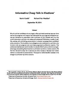
2.1 The different types of hypothetical bias in CE In essence, CT was originally intended to remove hypothetical bias by correcting for the nature of the hypothetical situation in a referendum CVM (Cummings and Taylor 1999). However, even though the CVM and CE methods are very closely related, there are important structural differences between the two methods that might consequently affect the effectiveness of CT. In CE respondents are typically asked to consider two hypothetical alternatives and a status quo (opt-out) alternative, in which the alternatives vary in multiple dimensions via the attributes, whereas in CVM they are most often asked to consider only one fixed hypothetical alternative and a status quo alternative. As the simplified schematic in figure 1 illustrates, this structural difference might lead to differences in the decision processes being invoked.

Improved situation (positive bid / ’Yes’) CVM

Status quo (zero bid / ’No’)

Alternative 1 Non-status quo

Alternative 1 CE1

Alternative 2

or

Alternative 2

CE2

Status quo (opt-out)

Status quo (opt-out)

Figure 1. Choice decision processes in CVM and CE.

In open ended CVM the decision is between stating a zero-bid (referendum: ‘No’) or some positive bid (referendum: ‘Yes’), i.e. the total WTP for the alternative situation. Hypothetical bias implies that the stated hypothetical WTP is higher than the real WTP (a higher percentage of ‘Yes’ responses in the hypothetical referendum than in the real referendum), i.e. WTPH > WTPR. CT is intended to lower the stated total WTP in CVM if hypothetical bias is present. Figure 1 presents two different choice decision processes that may be relevant in CE surveys. In CE1 the respondent considers all three alternatives simultaneously and chooses the one which maximizes her utility. CE2 suggests a slightly

5


different two-step decision process. The first step can be seen as the purchase decision where the respondent decides whether to stick with the status quo alternative or to opt for a nonstatus quo regardless of the attributes of these alternatives3. If the latter is chosen, the next step is choosing between the two proposed experimentally designed alternatives by considering the marginal values of the attributes. While CE1 is clearly a desirable decision process considering the basic theory underlying random utility theory, CE2 has some adverse implications. First, choosing the “non-status quo” route in the first step might be considered as strategic behaviour or even non-compensatory behaviour in the sense that the price attribute might be ignored which is in violation of the passive bounded rationality assumption and the continuity axiom4. Second, choosing the “status quo (opt-out)” route might reflect protest behaviour, though it may also reflect a genuine preference to stick with the status quo if the respondent is really not interested in any improvements. Considering these potential choice decision processes in CE, hypothetical bias would also lead to WTP being overestimated in CE, but here it might be so as a result of two different impacts. Firstly, marginal WTP for the attributes might suffer from hypothetical bias, i.e. MWTPH > MWTPR. Secondly, preferences for the opt-out alternative might be affected in the sense that hypothetical bias makes respondents dislike this alternative more than they would in real life, i.e. βH(OO) < βR(OO) 5. In other words, hypothetical bias could be present not only in the estimates of the marginal values of the attributes, but also in the purchase decision (List et al. 2006). In CE, the total WTP for some policy can be found by summing over the marginal WTPs for the relevant attributes as well as the (in the improvement case) WTP to avoid the opt-out alternative6. Thus, in CE it is possible to distinguish between three different types of hypothetical bias: 1) MWTPH > MWTPR and βH(OO) = βR(OO) 2) MWTPH = MWTPR and βH(OO) < βR(OO) 3

In the ”purchase decision” terminology this would be the WTP for the good regardless of its attributes. Here it is assumed that the “non-status-quo” alternatives present improvements on all attributes but the price attribute. 5 For protesters the opposite would be the case, i.e. βH(OO)> βR(OO), but these respondents are typically excluded from the analysis. 6 This very simple approach often used in practice applies to a “state-of-the-world” situation while a more theoretically consistent measure of welfare is put forth by Small and Rosen (1981). For a discussion on the appropriateness of the simple approach to calculating total WTP see Lancsar and Savage (2004) and the followup comments in Health Economics. 4

6


3) MWTPH > MWTPR and βH(OO) < βR(OO) Even though the decision processes might be quite similar, and in principle the three different types of hypothetical bias could just as well be present in CVM, it is clear that they cannot be distinguished from each other in CVM. Consequently, CT has traditionally not in any way been specifically targeted to address this issue of different types of hypothetical bias. Despite the fact that there are only a few studies in the CE literature testing for hypothetical bias in relation to total WTP and MWTP, there is some evidence in the literature that makes it relevant to consider the different types of hypothetical bias. In their beef steak experiment, Lusk and Schroeder (2004) find that hypothetical bias makes respondents report upwards biased probabilities of buying the good whereas marginal WTPs are not significantly affected. In other words, they identify the type 2 hypothetical bias. Similar results are found by Alfnes and Steine (2005). On the other hand, Ready et al. (2010), Taylor et al. (2007) and Broadbent et al. (2010) find evidence of both type 2 and type 3 hypothetical bias. List et al. (2006) also find evidence that the purchase decision can suffer from hypothetical bias both in a non-market and a market good case. As the non-market good case is a very simple CE experiment7, MWTP is not estimated and it is thus not possible to determine whether the hypothetical bias is of type 2 or 3. In the market good case they find evidence of type 2 hypothetical bias. Interestingly, they find that CT is able to remove hypothetical bias in both cases. However, the design of the very simple non-market good case is hardly representative of the majority of non-market CEs conducted in practice, so this result is probably not generalizable. While the CT does eliminate the type 2 hypothetical bias in the market good case, it has the adverse effect of introducing some internal preference inconsistency. To the authors’ knowledge, List et al. (2006) is the only published paper testing the effect of entreaties in relation to the three different types of hypothetical bias, so this is clearly an area for further investigation. 2.2 Out of sight, out of (the cognitively constrained) mind Another important structural difference that might be overlooked when simply adopting the CT approach directly from CVM, is the repeated choice nature of CE. In CVM, 7

Only one choice set per respondent is used, and all respondents receive the same choice set.

7


respondents are typically asked to answer one or two WTP questions, depending on the type of elicitation format. The CT script is presented to respondents in the scenario description preceding the WTP question(s). In CE, however, respondents are usually faced with a sequence of 4-12 choice questions after the scenario description. Thus, in terms of information processing, the average “mental distance” from the CT information in the scenario description to the valuation questions becomes longer in CE than in CVM. In practice this could translate into respondents forgetting about the CT information or at least paying decreasing attention to it in the later choice sets. If so, we would expect a decreasing impact of the CT and, consequently, potentially increasing hypothetical bias as respondents proceed through the sequence of choice sets. This would be expected regardless of which of the three types of hypothetical bias we are considering. Furthermore, the fact that respondents typically find CE to be more cognitively demanding than CVM might add to this in terms of increasing the speed with which the CT information is forgotten. There are several examples in the literature of how the effect of information on behaviour diminishes as the number of choice sets or tasks increase. In a study focusing on starting point bias in CE, Ladenburg and Olsen (2008) find that the bias caused by the price levels used in an instructional choice set appears to be reduced with the choice set number. In a study focusing on the same problem, Bateman et al. (2008) find that anchoring bias in CVM seems to be reduced as the respondent evaluates more and more evaluation questions. Similar results are found in Carlson et al. (2008b) who test the influence of conformity through information on the purchase of other consumers in a CE. In their paper, the information effects decrease insignificantly after completing the first four choice sets. These observations could suggest that the effectiveness of CT might be decreasing as a function of the number of choice sets, implicating that hypothetical bias of any type might increase as the respondent progresses through the sequence of choices and forgets about the CT information. The results in Ladenburg (2010) suggest that this actually might be the case. As previously mentioned, Ladenburg (2010) finds that the effect of a CT seems to be significantly reduced after three choice sets. On the other hand, several authors have found evidence of learning effects in CE (Bateman et al. 2008; Cherry et al. 2003; List 2003; Hutchinson et al. 2004; Ladenburg and Olsen 2008). This could suggest that the CT information simply becomes redundant as the respondent progresses through the choice sets and learns about own preferences. However, to the authors’ knowledge this specific relationship has yet to be tested in the literature.

8


Another difference between CE and CVM is the cognitive burden placed on respondents. In CVM, complexity and cognitive burden is related to the detailed descriptions of the current situation as well as the proposed policy change at some price. However, in CE it is furthermore related to the numbers of attributes, levels, alternatives and choice sets, and the experimental design typically focuses on maximum variation at the choice level. Arguably, answering a series of differing choice sets in a CE survey will most often be a more complex task than answering a single open ended or maybe two dichotomous choice questions in CVM survey. Several authors have found evidence of choice complexity in CE leading to seemingly irrational behaviour (Bradley and Daly 1994; Mazzotta and Opaluch 1995; Swait and Adamowicz 2001; DeShazo and Fermo 2002; Caussade et al. 2005). This issue is linked to the commonly assumed passive bounded rationality underlying choice behaviour. This carries the assumption that all respondents attend fully to all the available information for all choices made, but due to cognitive constraints respondents’ ability to make optimal choices decreases, as the information set increases (Puckett and Hensher 2008). Specifically, in a CE survey Puckett and Hensher (2008) find that increases in the amount of information presented leads to respondents enacting coping strategies to allocate their cognitive capital to subsets of the information rather than attending to the full set of information. These findings are in line with the “selective information processing” put forward by Meyers-Levy (1989). Specifically, if the information given to the respondents is not perceived to be sufficiently motivating or relevant for the respondent, the threshold for elaborating on the information might not be reached (Meyers-Levy and Maheswaran, 1991; Meyers-Levy and Sternthal, 1991). This introduces the risk that respondents – more or less intentionally – ignore the CT information as part of their coping strategy and information processing. Under the rather fair assumption that CE surveys are typically more complex and cognitive demanding than CVM surveys (Adamowicz et al. 1998), the risk of ignoring CT would be bigger in the CE context, ceteris paribus. Furthermore, as noted by List et al. (2006), CT is intended to make respondents correct for the hypothetical nature of the valuation question through an internal correction process where the respondent commits cognitive effort to reach a more accurate value statement. Assuming that cognitive capability is a not a limitless resource, CE surveys would leave less cognitive effort available for this CT instigated hypothetical bias correction process. This tendency might be even further exacerbated if respondents experience fatigue as they progress through the sequence of choice sets. A fatigue effect may trigger a coping

9


strategy which consequently involves ignoring the CT information. Thus, in CE, increasing fatigue might lead to decreasing attention being paid to the CT information as the number of choices increase, and, hence, we would expect hypothetical bias of any type to increase. This is clearly at odds with the passive bounded rationality assumption. 2.3. Relying on reversed conformity Another reason for potential ineffectiveness of CT, in CE as well as in CVM, is the specific wording of the CT scripts typically applied. The original CT script introduced in the CVM literature by Cummings and Taylor (1999) can be decomposed into three main parts according to the grammatical pronouns used: Firstly, it is described in a third person plural form how other respondents in previous surveys have disproportionally often voted “yes” in hypothetical referenda compared to actual referenda. This is explicitly dubbed “hypothetical bias”. In the second part, the first person singular form is used to describe potential explanations for this previously observed behavior. It is not until the last part of their script that Cummings and Taylor turn to the second person singular form and directly address the respondents with explicit instructions on how they themselves should act in the following referendum. Altogether it adds up to a very detailed and quite lengthy script consisting of about 500 words. In recognition of potential information overload, and to minimize the amount of reading required of the respondents, the CT scripts used in subsequent studies have typically been much shorter than Cummings and Taylor’s original script. This is of course not a problem per se, but typically these shorter scripts tend to focus mainly on the first part of Cummings and Taylor’s script – the part that addresses hypothetical bias only by mentioning that other respondents tend to be subject to it. However, if the last part of Cummings and Taylor’s script is left out, there is no explicit instruction to the respondents on how they themselves should choose, only the implicit instruction in the information about previous respondent’s erroneous choices. Thus, the focal point of information in the typical short CT script (and the first part of the original script in Cummings and Taylor (1999)) is that people in other stated preference surveys have overstated how much they would be willing to pay and thereby expressed a hypothetical bias in their choices. The effectiveness of the CT is thereby conditional on the respondent

10


perceiving the reported behaviour of others as inappropriate and, as a consequence, choosing to conform to the opposite behaviour8. The literature has several examples of conformity, i.e. how the individual’s decisions are governed by what other individuals do; see for example Frey and Meyer (2004); Shang and Croson (2007), Croson and Shang (2008), Alpizar et al. (2008) and Carlsson et al. (2008b). An imperative result from these studies is that upward and down ward social information make respondents conform to the direction of the information, i.e. conformity is parallel to the behaviour of others. However, considering the purpose of CT, the desired direction of the conformity is the opposite in the sense that the respondent is explicitly informed that what other people have done is inappropriate, implicitly carrying the message that the respondent should conform to the opposite behaviour. Besides the indirect tests in the CT literature, the issue of reversed conformity effects has not been given any attention in the experimental economics or behavioural psychology literature9. If we relate the reversed conformity properties of the CT to the process of choosing between the status quo alternative and the experimentally designed alternatives and the effectiveness of the CT, most of the previous economic experiments on social upward/down ward information have mainly focused on how social information influence whether or not to make a purchase on the hypothetical market and not how much (Croson and Shang 2008). An exception is the paper by Alpizar et al. (2008), which find that the level of social upward information can have dual effects on the demand. Information about other people’s demand for the good in focus can both influence the propensity to make a purchase but also the level of donation (conditional on the choice of donating) i.e. WTP. More specifically in a donation experiment they find that an increase in the level of demand in the upward social information reduced the purchase rate but increased the level of WTP conditional on purchasing. In relation to the effect of the CT on the three types of hypothetical biases, these results are noteworthy as they might give a more detailed insight into how CT might work in a typical CE experiment. If we use the Alpizar et al. (2008) view on a CE decision process, we would expect CT to push MWTP downwards. This is particularly evident in the present application, as we in our analysis condition attribute preference elicitation on market entrance. However, 8

Though we in this paper focus on short CT scripts, we would argue that the risk of not choosing to conform to the opposite behavior may also be present if using longer CT scripts in CE studies. 9 Our arguement is solely directed at the conformity literature. We acknowledge that the effects of warnings such as labels and ads are well established in the broader literature.

11


regarding the choice between the status quo/opt out alternative and the experimentally designed alternatives, the CT induced preference direction is less certain- does demand increase, decrease or is it not invariant? If we follow Alpizar et al. (2008) stringently in which the “participation rate/purchase decision” is negatively correlated with the direction of the social information, an increase in the propensity to choose an experimentally designed alternative could take place. Furthermore, being instructed on the subjection to hypothetical bias of other people might not be sufficiently motivating (Meyers-Levy and Maheswaran 1991) or of enough relevance (Hensher 2006) for the respondents to pay equal attention this piece of information throughout the sequence of choice sets. As such, a conformity link between the preferences of others and the preferences of the respondent might be relatively weak and potentially insufficient as a conveyer of the hypothetical bias mitigation information. The expected impact of CT on respondents in the form of a lower stated WTP can be interpreted as an economic behaviour which besides more traditional economic incentives also includes a wish to conform to the social norms, i.e. not to overestimate the level of WTP as put forward in the CT. However, as found in Carlsson et al. (2008b), the influence of conformity on stated behaviour is not necessarily homogeneous in a sampled population. In a study focusing on how information about other people’s demand for ecological coffee beans influence individual demand, Carlsson et al. (2008b) find that that male respondents do not express preferences that seem to be governed by a desire to conform to the demand by others. On the other hand, the preferences of the female respondents seem to express conformity characteristics. In a meta-analysis, Eagly and Carli (1981) also find differences in the way men and women conform to the behaviour of others. In the same line, Klick and Parisi (2008) state that people with low levels of risk aversion and high self-denial cost are less likely to conform. In Shang and Croson (2008) only respondents new on the field experiment market (donations to a public radio station) are affected by upward social information. Respondents who previously have made donations (renewing members) are not affected. In this perspective, it is questionable whether CT will actually induce the expected reduction of hypothetical bias uniformly across the sample as it relies to some degree on conformity effects. Especially when using the short script CT versions based exclusively on the first part of Cummings and Taylor’s script, this could pose a problem.

12


Finally it is also worth taking a closer look on the individual process of conforming. In the paper by Parisi and Klick (2008), conformity behaviour is presented to be a function of self-denial costs. More specifically, Parisi and Klick (2008) argue that an adaptation to information about others behaviour is not costless. More specifically, by adapting and conforming the initial set of preferences to the new set of preferences induced by the information about others, the individual will impose a cost associated with self denial. This has a negative influence on the propensity to conform, so that people with high self denial costs are less likely to conform. If we apply this theoretical framework in the CE setting, we would have to assume that self denial costs are constant across the choice sets in order for the CT to have a uniform effect in all the choices. A study by Shroeder et al. (1983) suggests that this might not be the case. In a social trap game, participants received different types of real and manipulated information on the behaviour of the other participants in the first three blocks of the experiment. As found in the other conformity studies mentioned, people conformed to the behaviour of other participants. However interestingly, as soon as the information was stopped, the conforming behaviour also stopped. In this light, we would expect that the respondents might not pay equal attention to the CT across all choice sets in a CE survey. 3. The Opt-Out Reminder experimental setup To mitigate some of the above mentioned potential shortcomings of CT in CE, the OOR is first of all intended to enhance the effectiveness of short CT scripts by directing the respondent’s attention to the trade-off between attributes and cost with the opt-out alternative as an explicit benchmark. The goal is thus to reduce any remaining hypothetical bias which CT has failed to remove. Especially the types of hypothetical bias which are related to the propensity to make a purchase at the hypothetical market should be reduced, ideally to an extent where βH(OO) = βR(OO). As argued, CT might have difficulties dealing with this specific element in the CE decision process, especially if the respondent uses a decision process similar to CE2 in figure 1. The OOR works by simply reminding the respondents that it is perfectly okay to choose the opt-out alternative if they find the other alternatives too expensive. The exact wording of the OOR used in the empirical survey (also in appendix 1) is the following:

13


“If both prices are higher than what you think your household will pay, you should choose the present situation (the opt-out).” First of all, the reminder turns the respondent’s attention to the trade-off between the optout alternative and the experimentally designed alternatives, thereby attempting to mitigate the type 2 and 3 hypothetical bias. The second aim of the OOR is to accommodate for the repeated choice structure in CE. The OOR is applied in a dynamic setup by presenting it to the respondents not just once, but prior to each single choice set. By adding a dynamic reminder to the static CT we aim to ensure that equal attention is paid to this information throughout the sequence of choice sets. In other words, respondents are continually reminded not to let their answers become hypothetically biased. While the CT information provided in the scenario description might be very present in the respondent’s mind in the first choice sets, it seems likely that it will be less so in the later choice sets. As a consequence, we might see increasing hypothetical bias in the later choice sets in a CE using a short CT script. If this is indeed the case, then adding a dynamic OOR could serve as a remedy to this problem by repeatedly reminding respondents to stay on the “true” preference path regardless of the number of choice sets. Finally, the reminder does not rely on conformity effects as it asks the respondents explicitly to make a judgement themselves with regard to whether the experimentally designed alternatives are too expensive or not. The wording used in the OOR is thus in the second person singular form, thus re-introducing the more direct and personal approach used in the third part of Cummings and Taylor’s original CT script. We expect that such a more direct and explicit instruction will make a stronger impression on the respondents. Consequently, it could be more effective in reducing hypothetical bias, especially in the case of cognitively demanding CE surveys where CT applied alone might come short. Similar to Aadland and Capland (2003), Bulte et al. (2005), Carlsson et al. (2005) and Lusk (2003), we apply two hypothetical treatments in otherwise identical environments to isolate the potential effect of the OOR. The only difference between treatments is that in one treatment respondents are provided with an OOR before each choice set (the “OOR” sample) whereas they are not in the other (the “NOOR” sample). Both samples are given identical short CT scripts provided as a one-shot piece of information implemented in the scenario description prior to the sequence of choice sets. The CT used in the empirical survey is a very

14


short version focusing solely on the first part and the budget reminder part of Cummings and Taylor’s original CT script. The exact wording is as follows: “Remember to consider how the additional yearly tax payment will affect your household’s disposable income for other purposes. In similar surveys it has been found that people tend to overestimate how much they would really be willing to pay.” This experimental setup calls for a couple of remarks. First of all, we are not suggesting completely abandoning the use of CT and using OOR instead. Assuming that a short CT script in the scenario description on its own is not sufficiently effective in removing both the marginal and total hypothetical bias in CE, our hypothesis is that augmenting it with the dynamic and direct OOR will adapt the CT to the CE structure and make it more effective in terms of reducing stated WTP, marginal as well as total. If confirmed, this would suggest that the reminder could be effective against all three types of hypothetical bias. Secondly, as this is a non-market good case, comparable real market data are unfortunately not available. This is a well-known limitation in applications considering these types of goods (Aadland and Capland 2003, Bulte et al. 2005, Carlsson et al. 2005, Lusk 2003). As a consequence of this experimental setup we cannot assess the actual level of hypothetical bias present in our data. It follows that we are not able to test per se whether our CT treatment has actually completely eliminated hypothetical bias on its own and any further reduction of WTP due to the addition of the OOR would consequently lead to an underestimation of the true WTP.. What we can test with our experimental setup, is whether adding the OOR leads to significant reductions in MWTP and total WTP and whether such reductions vary systematically, i.e. as a function of the choice set number. Considering the previous findings in the literature concerning hypothetical bias and CT in CE, it does not seem farfetched to see our experimental setup as a test, not only of the presence of hypothetical bias after applying CT and in particular the longevity of CT in a choice set sequence, but also of which specific type of hypothetical bias it is. 4. The empirical survey The empirical survey is based on a questionnaire aimed at surveying local citizens’ preferences for a public good, in our case streams in urban green areas. In particular, the survey aimed at examining preferences for re-establishing a stream, Lygte Å. The stream is

15


currently running in an underground pipeline through an urban park, Lersøparken, located in a densely populated area of Copenhagen. Respondents were recruited from the population living in the three Copenhagen city districts Bispebjerg, Nørrebro and Østerbro, all located adjacent to Lersøparken10. From each city district, 2x200 respondents between the ages 18 and 70 were randomly drawn from the Danish Civil Registration System (DCRS), summing up to a total of 1200 respondents, who were mailed a self-administered questionnaire. The construction and validation of the questionnaire was carried out firstly by approaching people visiting Lersøparken in an informal manner, asking them about their perceptions and attitudes towards a potential re-establishment of the stream. Secondly, four focus groups were interviewed as part of developing the questionnaire and identifying the relevant attributes and attribute levels. The final set of attributes used in the CE design as well as the associated attribute levels are displayed in table 1. Table 1. Attributes and attribute levels Attribute Course of the stream

Levels Straight Meandering Water level One month dry-out per annum no dry-outs Stream edges/banks Covered with flagstones Covered with grass Stream profile Single Double Price (tax increase) 50, 100, 200, 400, 700 and 1100 DKK/household/year Note: DKK100 ≈ €13.4 ≈ US$16.2

Coding 0 1 0 1 0 1 0 1 Continuous

A D-optimal fractional factorial design was generated entailing a total of 24 experimentally designed alternatives. The alternatives were paired into 12 choice sets which were randomly blocked in two. Consequently, each respondent evaluated six choice sets in total. Besides the two experimentally designed alternatives, each choice set contained a third alternative; the opt-out alternative, which entailed leaving the stream in the current pipeline at no extra cost. See Appendix 1 for an example of a choice set. An accompanying A3-size information sheet was provided showing photo-realistically manipulated colour visualizations of all attributes and levels. Furthermore, an A4-size colour sheet with a map of the park area 10

The associated benefits were expected to be strongly dependent on the use of the park, hence, the geographical delimitation of the target population.

16


and pictures of the current situation was enclosed in the mail-out envelope. These visualizations were provided to increase the level of comprehension and evaluability of the attributes (Bateman et al. 2009; Boyle 2003; Mathews et al. 2006). 5. Econometric specification To test for equality of preferences across treatments we apply a random utility function. Let individual i’s utility of choosing alternative j be given by: Uij = Vij + εij, where Vij is the systematic part of the utility associated with the stream attributes and εij is a stochastic element. Assuming Vij is linear in parameters, the systematic utility of alternative j can be expressed as: Vij = β’Xij + φAij+ η’Pij. The β’s are the coefficients representing the utility associated with the attributes, Xij, of the re-established stream, φ is the coefficient associated with the alternative specific constant for the opt-out alternative, Aij, representing the utility of the opt-out alternative relative to the re-establishment alternatives, and, finally, η represents the (dis-)utility of the price, Pij. The probability of an individual choosing alternative j from a choice set consisting of alternatives, j, k and l is given by: Prob(Vij + εij> Vik + εik, Vij + εij> Vil + εil). A mixed logit model which incorporates random parameters as well as an error component was found suitable for the parametric analysis of preferences. This Random Parameter Error Component Logit (RPECL) model allows for panel specification which captures the repeated choice nature of the data set explicitly in the model (Train 2003). Furthermore, the random parameters specification allows explicitly for unobserved taste heterogeneity, i.e. random taste variations across respondents, and it is not restricted by the Independence of Irrelevant Alternatives (IIA) assumption (Hensher and Greene 2003; Revelt and Train 1998; Train 2003). Specifically, parameters associated with the attributes of the reestablished stream are specified as normally distributed random parameters to allow for both negative and positive preferences for the physical attributes of the stream. Focus group interviews and a pilot test indicated that this could be expected. The multivariate normal distribution of individual tastes across individuals can be written as β n ~ N ( β , Ω). The variance-covariance matrix Ω is specified so as to allow for correlation across random parameters, i.e. diagonal as well as off-diagonal values are estimated in the model (Train and Weeks 2005; Scarpa et al. 2008).

17


The price parameter is treated as a fixed rather than a random parameter, even though it implies fixed marginal utility of money. This approach is chosen for two reasons. First, it results in a behaviourally plausible negative sign for all respondents, and it allows for a relatively simple estimation of the distribution of marginal WTPs (Carlsson et al. 2003). Secondly, and more importantly, it avoids a number of severe problems associated with specifying a random price parameter (for further details, the reader is referred to e.g. Meijer and Rouwendal 2006; Hensher et al. 2005; Hess et al. 2005; Train and Sonnier 2005; Campbell et al. 2006; Hensher and Greene 2003; Rigby and Burton 2006; Train 2003; Train and Weeks 2005). Following Scarpa et al. (2005) an Alternative Specific Constant (ASC) is specified for the opt-out alternative in order to capture the systematic component of a potential opt-out effect. This is treated as a non-random parameter. Furthermore, an error component additional to the usual Gumbel-distributed error term is incorporated in the model to capture any remaining opt-out effects in the stochastic part of utility. The error component which is implemented as an individual-specific zero-mean normally distributed random parameter is assigned exclusively to the two experimentally designed alternatives. By specifying a common error component, correlation patterns in utility over these alternatives are induced. Thus, it captures any additional variance associated with the cognitive effort of evaluating experimentally designed hypothetical alternatives (Greene and Hensher 2007; Scarpa et al. 2007; Scarpa et al. 2008). 6. Results and Discussion 6.1 Response rates and respondent demographics Of the 1200 questionnaires sent out, 587 were returned with all questions answered. Table 2 presents an overview of certain descriptive statistics of the returned questionnaires. Initially, quite similar response rates of just below 50% were obtained in both split samples. However, based on follow-up questions, protest zero bidders11 and strategic bidders12 were identified and removed from the data. Further, serial opt-outers, defined as respondents who 11

Protest zero bidders were identified as respondents who chose the opt-out alternative in all six choice sets and in follow-up questions reasoned these choices with “I think the stream should be re-established, but I don’t want to pay more taxes” or “I cannot assess how much more I would be willing to pay in extra taxes”. 12 Strategic bidders were identified as respondents who in all six choice sets chose one of the experimentally designed alternatives and reasoned it with “I didn’t consider the tax payment at all” or “I have not considered the tax payment, but I want to affect the policy decision”.

18


chose the opt-out alternative in all six choice sets, were excluded from the analysis13. Accordingly, the effective response rates associated with the samples used in the following analyses is 24.2% for the NOOR sample while it is 29.2% for the OOR sample. Conditional on this setup, the parametric analysis is based on a total of 145 respondents in the NOOR sample and 175 respondents in the OOR sample.

Table 2. Descriptive statistics of obtained responses NOOR

OOR

Questionnaires sent out - No reply - Protest zero bids - Strategic bids - Serial opt-outers Sample used for analysis

# 600 309 36 85 25 145

% 100.0 51.5 6.0 14.2 4.2 24.2

# 600 304 34 67 20 175

% 100.0 50.7 5.7 11.2 3.3 29.2

No. of choices in data Occasional opt-out choices in data

870 199

100.0 22.9

1050 380

100.0 36.2

Table 2 shows that the OOR sample does not obtain a higher number of protest zero bidders than the NOOR sample. This is interesting, as one might have suspected that by introducing the OOR we would run the risk of introducing or increasing an opt-out bias in terms of respondents disproportionally often choosing the opt-out alternative (Samuelson and Zeckhauser 1988; Hartman et al. 1991). Meyerhoff and Liebe (2009) summarize four different reasons for choosing the opt-out alternative in CE: 1) Genuine preferences, 2) protest beliefs, 3) heuristic to overcome complexity, and 4) zero-price effects. While the first reason would imply that an observed choice of the opt-out alternative reflects a true preference for this alternative, any of the last three reasons would imply that the choice is biased. In the light of this, and the fact that the OOR treatment in our case actually results in slightly fewer protest zero bidders as well as fewer serial opt-outers, the suspicion of

13

Exclusion is an often used way of dealing with serial opt-outers (Alfnes et al. 2006; Burton and Rigby 2009). This approach has been criticized by von Haefen et al. (2005) and Lancsar and Louviere (2006) in part for assuming seperability. However, Burton and Rigby (2009) find that accounting for serial opt-outers rather than simply excluding them only leads to minor changes, and they conclude that relatively little is lost in taking the conventional approach in terms of excluding serial opt-outers.

19


increased opt-out bias in the OOR sample cannot be confirmed14. However, as the lower part of table 2 shows, the OOR sample obtains a markedly higher share of occasional opt-out choices, i.e. where the respondent in at least one of the other choice sets has chosen an experimentally designed alternative. As such, it is not surprising that the introduction of the OOR results in an increased propensity to choose the opt-out. This might suggest that the OOR has made respondents consider their preferences more closely when choosing, and as a consequence, their choices are less influenced by hypothetical bias especially in the purchase decision. The fact that the number of strategic bidders is apparently somewhat lower in the OOR sample is in support of this interpretation. This is however not strong evidence, so a more thorough parametric analysis of the stated preferences is conducted in section 6.2. The datasets obtained from the NOOR and the OOR samples are based on choices from two independent samples from the population. Differences in demographic background characteristics between the two samples might weaken the potential for inference with regard to the effect of the OOR, unless explicitly accounted for. Hence, before observed differences in preferences can be assigned to the effect of the OOR, it has to be ascertained whether the respondents in the two samples differ with regard to their demographic background characteristics. Table 3 reports summary statistics for a few selected demographic characteristics. Pearson χ2-tests applied within each of these categories cannot reject the null hypothesis of equality of distributions across split samples in any of the cases. This suggests that the two respondent samples on average are homogeneous with regard to demographic characteristics15. Thus, if a difference in preferences across the two samples is established in the following analyses, it can more likely be ascribed solely to the OOR. Furthermore, the fact that the two samples are close in terms of covariates makes it reasonable to look at unconditional WTP estimates when comparing WTP across samples.

14

For a more detailed description of the potential effects of pre-amples/scripts to reduce protest zero bids, see Bonnichsen and Ladenburg (2009). 15 Tests have been carried out for a wider range of demographic categories than presented in table 2. These are available from the authors on request. All of these support the overall conclusion that the two samples do not differ significantly with regard to demographic background characteristics.

20


Table 3. Descriptive statistics of sampled respondents

Demographic categories Gender Male Female Age 18-29 30-39 40-49 50-59 60-70 Education Elementary school Upper Secondary Vocational Education Higher Education (1-2 years) Higher Education (2-4years) Higher Education (>4 years) Household net income per year < 150,000 DKK 150,000 – 399,999 DKK > 399,999 DKK Local city district Bispebjerg Nørrebro Østerbro Total number of respondents

Sample NOOR OOR 49.7% 50.3%

52.6% 47.4%

40.0% 30.3% 9.7% 13.1% 6.9%

40.0% 33.1% 11.4% 10.3% 5.1%

5.6% 9.7% 9.0% 8.3% 28.5% 38.9%

6.9% 9.7% 5.1% 8.0% 26.3% 44.0%

27.6% 40.7% 31.7%

24.0% 38.9% 37.1%

30.3% 33.8% 35.9%

31.4% 30.3% 38.3%

145

175

6.2 Parametric Analysis Hausman and McFadden (1984) tests clearly rejected the assumption of proportional substitution across alternatives, i.e. the IIA property. Hence, we do not present MNL models as these do not allow for violations of the restrictive IIA assumption. Instead, the parametric modelling of choices is carried out using the less restrictive RPECL model described in section 5. The RPECL models have been analysed using Nlogit 4.0. As no closed form solutions exist for the RPECL models, they are identified using simulated maximum likelihood estimation with 300 Halton draws which was found to be a sufficient number to obtain stable results. The results are displayed in table 4.

21


Table 4. Random parameter error component model estimates. Absolute values of tstatistics in brackets. Parameter estimates

Model 1 NOOR OOR

Model 2 NOOR OOR

1.368 (5.53) 1.172 (4.43) 1.595 (6.78) 0.649 (3.00) -0.007 (17.20) -1.460 (4.11) -

1.484 (5.81) 0.735 (3.51) 1.610 (6.09) 0.513 (2.32) -0.009 (17.08) -0.459 (1.87) -

1.003 (3.22) 0.859 (2.11) 1.131 (2.98) 0.436 (1.53) -0.006 (15.18) -4.191 (3.94) -1.884 (2.34) -1.873 (2.51) -1.811 (2.95) -1.617 (3.64) -3.901 (2.77)

1.124 (3.74) 0.630 (1.88) 1.311 (3.83) 0.406 (1.33) -0.008 (14.21) -2.805 (4.26) -0.189 (0.36) -0.502 (0.84) 0.121 (0.25) -0.762 (2.25) -1.497 (1.40)

1.168 (4.48) Water level 1.467 (6.09) Grass banks 1.186 (5.35) Stream profile 0.807 (2.85) Error component parameters 2.485 σ12 (4.96)

1.371 (5.61) 1.113 (3.38) 1.442 (5.03) 1.195 (3.50)

1.197 (4.12) 1.370 (5.15) 1.304 (4.76) 0.834 (2.74)

1.227 (4.96) 0.830 (1.88) 1.266 (4.03) 1.055 (2.96)

2.064 (6.09)

2.694 (4.68)

2.135 (5.53)

Means Meandering Water level Grass banks Stream profile Price ASC(OO) ASC(OO) - CS1 ASC(OO) - CS2 ASC(OO) - CS3 ASC(OO) - CS4 ASC(OO) - CS5 ASC(OO) - CS6 Standard deviations Meandering

Log Likelihood -579 -713 -568 -694 No. of observations 870 1050 870 1050 Adjusted McF. R2 0.39 0.38 0.40 0.39 LR-test statistic 30.2* 29.1 Note: For the LR-test statistic ‘*’ denotes significance at 0.05 level.

22


We apply two different specifications. The first specification (Model 1) is as described in section 5. The second specification (Model 2) elaborates on the first by estimating choice set specific ASCs rather than a single overall ASC for the opt-out alternative. This is done in order to test for a potentially increasing or decreasing effect of the OOR on the preferences for the opt-out alternative. As mentioned in section 2, this could be caused by respondents forgetting the CT information as they progress through the sequence of choice sets, or it could be a consequence of learning or fatigue effects. In general, the parameter estimates reveal that respondents have significant preferences for improving the physical condition of the re-established stream from the low (zero) to the high (one) levels. Thus, the respondents prefer a meandering stream over a straight stream; a stream with constant water flow rather than a stream which periodically dries out; a stream with grass banks rather than flagstones; and a double profile stream rather than a single profile stream. The internal ranking of stream attributes is similar in both samples. Respondents show the strongest preferences for “Grass banks”, followed by “Meandering” and “Water level” attributes, whereas the “Stream profile” is less important and even insignificant in model 2. All standard deviation parameter estimates for the random components are significant. This reveals that there is significant and similar degree of preference heterogeneity in both samples. As expected, the estimate for the price parameter is negative across all models in table 4.

Table 5. Cholesky matrix (lower triangular and diagonal, absolute t-values in brackets) and correlations (upper triangular) for model 1 on the OOR sample. Meandering Water level Meandering 1.371 0.099 (5.61) Water level 0.111 1.108 (0.33) (3.46) Grass banks 0.130 -0.571 (0.42) (1.77) Stream profile -0.734 0.926 (2.33) (2.65)

Grass banks 0.090

Stream profile -0.614

-0.385

0.709

1.318 (4.71) -0.169 (0.30)

-0.491 0.075 (0.05)

23


The RPECL model allows for a full correlation structure across the random parameters. From the accompanying estimated correlation matrix and Choleski matrix in table 516, we see that there is negative correlation between preferences for “Water level” and “Grass banks”, as well as between “”Meandering” and “Stream profile”, while there is a significantly positive correlation between preferences for “Water level” and “Stream profile”. With regard to possible differences in preferences between the two samples, the parameter estimates are not directly comparable across models due to potentially differing scale parameters in the two samples (Louviere et al. 2000). Nevertheless, flicking through the parameter estimates17, signs, magnitudes and levels of significance are quite similar for the two samples, suggesting that the OOR does not affect the marginal utility of the stream attributes much. The alternative specific constant ASC(OO) in model 1 expresses the utility associated with the opt-out alternative relative to the two re-establishment alternatives. This utility is attributed to the opt-out alternative in itself and cannot be explained by other explanatory variables in the model18. Interestingly, the significantly negative sign of the ASC estimate in model 1 suggests that an opt-out effect is present, but it is the reverse of what is usually observed. Typically, respondents tend to choose the opt-out alternative disproportionally often, leading to a positive ASC estimate (Samuelson and Zeckhauser 1988; Hartman et al. 1991; Rabin 1998; Meyerhoff and Liebe 2009; Adamowicz et al. 1998). However, the negative ASC estimates found in the current study indicate that respondents have a strong aversion toward the opt-out alternative regardless of how desirable the experimentally designed alternatives are. In other words, respondents are inclined to support a reestablishment of the stream, ceteris paribus. The results in model 2 confirm that this apparent reversed opt-out effect is present throughout all six choice sets. According to Lehtonen et al. (2003) and Scarpa et al. (2005) who find similar results, this would be consistent with a 16

Table 5 only reports the results obtained in model 1 for the OOR sample. As the remaining three correlation and Cholesky matrices show very similar results, they are left out for simplicity. 17 We argue that comparisons between the parameter estimates are not completely inappropriate here, as we find only very small and insignificant differences in scale factors. 18 According to Meyerhoff and Liebe (2009) the interpretation of the ASC parameter depends on whether one sees it mainly as a technical parameter capturing the average effect of all relevant factors that are not included in the model, or one chooses to associate the ASC parameter with a behavioral assumption. As suggested by Adamowicz et al. (1998), we choose the latter approach and interpret the ASC(OO) as the utility of the opt-out alternative.

24


perception of under-provision of the public good under evaluation. The negative ASC could of course reflect a true preference to change the current situation in the park, but it could also be interpreted as evidence of hypothetical bias that is not removed by the CT. If indeed present, behavioral reasons such as “warm glow”, “positive self-image” and interviewer bias are likely to materialize in the experimentally designed alternatives being chosen disproportionally often over the opt-out alternative. If the latter interpretation is relevant, we would expect the introduction of the OOR to reduce hypothetical bias of type 2 or type 3 and, consequently, result in an increase in the ASC estimate. Turning to the ASC estimate in the OOR sample, this is exactly what we find. In model 1, the ASC is still negative but now numerically smaller and no longer significantly different from zero at the 95% confidence level. This suggests that the reversed opt-out effect observed in the NOOR sample actually constitutes a hypothetical bias rather than a genuine preference structure. These results support the usefulness of the OOR in CE, as they indicate that the OOR may indeed assist CT in more effectively reducing hypothetical bias type 2 or type 3. Though less clear cut, the OOR appears to have had similar effects at the choice set level in model 2. Here, it is evident that most of the choice set specific ASCs are significant in the NOOR sample, while the majority of the ASCs are higher (less negative) and insignificant in the OOR sample. This supports the findings from model 1 that in the OOR sample, there is a stronger tendency for respondents to no longer want a re-establishment of the stream unless they have some saying on the physical attributes of the stream. The fact that the choice set specific ASCs in model 2 seem to differ pair wise across the two samples, would suggest that the effect of the OOR persists throughout the sequence of choices. It is however not possible to say whether the effect is constant or rather slightly decreasing or increasing. While the ASC captures the deterministic part of the opt-out effects, the error component captures the stochastic part of the opt-out effects by estimating the covariance between the utilities of the two re-establishment alternatives relative to the utility of the opt-out alternative (Scarpa et al. 2005; Scarpa et al. 2008). In both models, the error component covariance estimates identify substantial positive correlation amongst the experimentally designed alternatives. The correlation in the NOOR sample is 0.76 and 0.82 for models 1 and 2, respectively, while it is slightly lower in the OOR sample at 0.72 and 0.74. Looking at the total variance of the utility for these alternatives (8.12 and 8.90 in the NOOR sample for models 1 and 2, respectively, and 5.91 and 6.20 in the OOR sample), it is clearly much higher

25


than the Gumbel error variance of π2/6 ≈ 1.645 which is assumed for the opt-out alternative. Interestingly, the total variance of the utility of the experimentally designed alternatives is 2730% lower in the OOR sample than in the NOOR sample. This suggests that the OOR reduces not only the deterministic part of the opt-out effect, but also the stochastic part. Altogether, this could be interpreted as an indication that the OOR does indeed make respondents pay more attention to the attributes and consider their tradeoffs relative to the zero-priced opt-out alternative more closely and in accordance with their true preferences. Looking at the Log Likelihood values, it is evident that model 2 provides a slight but nevertheless significant improvement to model 1 for both samples. This is also supported by increases in the adjusted McFadden pseudo-R2 values.

Table 6. Comparison of WTP estimates across samples Mean marginal WTP (DKK) Meandering Water level Grass banks Stream profile ASC(OO) ASC(OO) - CS1 ASC(OO) - CS2 ASC(OO) - CS3 ASC(OO) - CS4 ASC(OO) - CS5 ASC(OO) - CS6

NOOR 190 163 222 90 -203 -

Model 1 OOR P-value a 169 0.303 84 0.03 183 0.176 58 0.207 -52ns 0.003 -

NOOR 155 133 175 67ns -648 -291 -290 -280 -250 -603

Model 2 OOR 147 83 172 53ns -368 -25ns -66ns 16ns -100 -196ns

P-value a 0.447 0.251 0.483 0.403 0.078 0.031 0.059 0.005 0.032 0.063

a

P-values report results of the one-sided t-test that WTPNOOR > WTPOOR for each corresponding parameter. Variances of the mean WTP point estimates were calculated using the Delta Method as described in Greene (2003) and Hanemann and Kanninen (1999). ‘ns’ indicates that WTP estimates do not differ significantly from zero at the 0.10 confidence level.

A more formal test of the hypothesis of identical preferences in the two samples is reported in the last row of table 4. This is the Likelihood Ratio (LR) test for pooling datasets with identical data generating processes. The null hypothesis of equal preferences across samples is tested by pooling the two samples after having controlled for scale differences

26


(Swait and Louviere 1993; Louviere et al. 2000). The results of the LR tests indicate that on the overall preferences differ across the NOOR and OOR samples19. Elaborating further on the particular differences in preferences across the two samples is done by comparing the WTP estimates displayed in table 6. Calculation of WTP entails cancelling out the scale parameters, thus enabling direct comparison between the two samples (Louviere et al. 2000). It is evident that there is a tendency for MWTP estimates for the four stream attributes to decrease numerically when introducing the OOR. However, this reduction of MWTP when moving from the NOOR to the OOR sample is only significant for the “Water level” attribute in model 1. This confirms that the OOR has had some but not much effect on the MWTP for the specific attributes of the re-established stream. Turning to the ASC WTP estimates, significant differences appear. In model 1, the ASC WTP is negative and significantly different from zero in the NOOR sample, but when introducing the OOR we see a significant change in the preference for the ASC, resulting in a negative WTP which is no longer significantly different from zero. In relation to the previously discussed reversed opt-out effect, this increase in the ASC WTP implies a decrease in the aggregate welfare measure for any re-establishment of the stream20. Assuming that CT has not been effective in removing hypothetical bias in the NOOR sample, and, hence, welfare estimates are per se overestimated, this confirms that the OOR can prove helpful in obtaining lower value estimates which are less prone to type 2 or type 3 hypothetical bias. The fact that we only find relatively small differences in MWTPs suggests that CT on its own has to a large extent reduced hypothetical bias in these, even though our experimental setup does not allow for a formal test of this. This would entail that CT might be effective against hypothetical bias type 1, whereas the significant differences in ASC estimates suggests that CT is ineffective when it comes to types 2 and 3. Model 2 further confirms this tendency as significant increases are found for all choice set specific ASCs while the differences between the attribute MWTPs across samples become less outspoken, though still uniformly decreasing from the NOOR to 19

Only minor and insignificant differences with regard to the scale factors were identified in the LR test procedures and they are thus not reported here. As the additional five parameters in model 2 increase the degrees of freedom for the LR test statistic from 17 to 22, the critical value at the 0.05 significance level also increases to a value of 33.92. Hence, for model 2, the LR-test cannot actually reject the hypothesis of statistically identical preferences. 20 Reversing the sign of the estimated WTP provides the (now positive) WTP associated with a change from the current situation to a situation with a re-establishment of the stream regardless of the physical attributes.

27


the OOR sample. This confirms the findings from table 4; the OOR apparently does have a significant effect throughout the sequence of choice sets. While this result is maybe not surprising considering the fact that the OOR is displayed in each single choice set, it positively confirms that respondents have noticed it and paid attention to it in all choice sets. It is however still difficult to say whether the impact of the OOR is constant over the choice sets, or it is decreasing as a consequence of learning effects or maybe rather increasing due to fatigue effects or respondents paying decreasing attention to the CT information as they progress through the sequence of choices, as found in Ladenburg (2010). To explore these matters in more detail, we divide our original datasets into four subsets. Each of these contain data from only three consecutive choice sets with the first consisting of data from choice sets 1, 2 and 3, the next consisting of data from choice sets 2, 3 and 4, and so on. Due to the size of the data set, it is not possible to run a fully specified RPECL model. As an alternative, we therefore apply a somewhat simpler Random Parameter Logit (RPL) model. The RPL model is specified by allowing for heterogeneity in preferences for all the main attributes and the ASC(OO). All random variables are assumed normally distributed and the price variable is fixed. Again, simulations are based on 300 Halton draws. With these models, we set up a test for potentially evolving differences in preferences as a function of the choice set sequence. We thereby get a measure of the relative effect of CT on its own versus CT augmented with the OOR over the sequence of choices. Assuming a constant effect of the OOR and a decreasing effect of the CT, we would expect to find increasing differences in preferences between samples when moving from the first to the later choice sets. In table 7 we present three tests of identical preferences. In the first column, a LR-test allowing for differences in scale parameters is presented. In the next three columns, the mean total WTP for re-establishing the stream is estimated for each sample, and the differences in total WTPs are calculated. In the latter, for the attributes for which it cannot be rejected that MWTPNOOR> MWTPOOR, the levels of significance are also reported in superscript. Starting with the LR-test statistics in table 7, the test results indicate that stated preferences in the OOR and NOOR samples cannot be rejected to be identical in the first three choice sets used in the survey. In other words, adding the OOR seems to have had no significant impact in this first sequence of choices. However, moving to the models based on the later choice set (2, 3, 4), (3, 4, 5) and (4, 5, 6), significant differences in the preferences are found. The estimated levels of total WTP shed further light on the properties of these

28


differences in preferences. As reported in the fourth column, differences in total WTP are not significant in the three first choice sets. However, as the respondents evaluate more choice sets, the total WTP in the NOOR samples increases from 684 DKK in choice set (1, 2, 3) to between 841-938 DKK in choice sets (2, 3, 4), (3, 4, 5) and (4, 5, 6), whilst being relatively stable or even decreasing in the OOR sample. In more details, the levels of total WTP in the OOR sample are 610 in the first three choice sets and between 357-546 in choice set (2, 3, 4), (3, 4, 5) and (4, 5, 6)21. Interestingly, the differences in total WTP are found to be significant in choice sets (2, 3, 4), (3, 4, 5) and (4, 5, 6). In other words, WTP estimates in the OOR sample do not seem to increase as a function of the number of choice set, whereas this appears to be the tendency in the NOOR sample. First of all this suggests that the CT applied in the NOOR sample relative to the OOR sample has had a diminishing effect on the demand for re-establishing the stream throughout the sequence of choices. This speaks in favour of our suspicion that CT might only be capable of reducing hypothetical bias in the first choice sets in a CE which is also in accordance with the findings of Ladenburg et al. (2010). Apparently, respondents tend to forget about this piece of information as they move further away from the scenario description. This could explain why CT might decrease the internal consistency as found in List et al. (2006). Secondly, the non-increasing level of total WTP in the OOR sample indicates that the OOR has had an effect. These findings suggest that repeating the reminder might be crucial in order to induce hypothetical preferences that are in line with real preferences across all choice sets. One proposal could be to repeat the CT with each choice set. However, even with very short CT scripts, this might be too tiresome for the respondents to read and relate to, and undesirable fatigue effects might appear. Finally, as argued, CT itself might not be able to accommodate for hypothetical bias types 2 and 3. Given the results, we therefore argue that the inclusion of the OOR jointly with a CT might be an effective tool to remedy hypothetical biases associated with the marginal and total WTP across the entire choice set dimension in CE.

21

As the choice set order was not randomized, within split-sample comparison between choice sets is not valid in the sense that the properties of the design in the first three choice sets are different than the design properties in choice sets 2,3 and 4, choice sets 3,4 and 5 and choice sets 4,5 and 6. Despite this, comparisons of tendencies in these subset WTP estimates across the two split samples are valid as the choice set sequence was identical in the two split samples.

29


Table 7. LR-tests for identical preferences and WTP estimates across subsamples. Dataset based on choice sets: 1, 2 and 3c 2, 3 and 4 3, 4 and 5 4, 5 and 6

LR-test statistic (DF) 11.7 (11)NS 27.5 (11)*** 29.3 (11) *** 29.4 (11) ***

Total WTPOORa 610 546 357 507

Total WTPNOOR 684 938 841 889

Diff. Total WTPb

NS, -

-74 392*, -483***, Grass Banks**, ASC(OO)** -382***, ASC(OO)***

Note: ‘*’ indicates significance at 0.10 confidence level, ‘**’ at 0.05 level and ‘***’ at 0.01 level. ‘NS’ indicates that WTP estimates do not differ significantly from zero at the 0.10 confidence level. a The total WTP is estimated by summing the WTPs for all the attributes in the specific choice set models including the value attached to the ASC for the opt-out, i.e. ASC(OO). b In superscript, the attributes for which the one-sided t-test cannot reject that WTPNOOR > WTPOOR are reported. Variances of the mean WTP estimates were calculated using the Delta Method as described in Greene (2003) and Hanemann and Kanninen (1999). c For model identification purposes, the Stream Profile attribute had to be modeled as a fixed parameter in the first subset of choice sets.

7. Conclusion It has become more or less common practice to include Cheap Talk (CT) in stated preferences studies in order to reduce hypothetical bias. However, a considerable amount of studies have tested the effectiveness of CT in Contingent Valuation (CVM) and found that it might not be entirely effective in removing hypothetical bias. Few studies have dealt with the subject in Choice Experiments (CE), but also here the results are ambiguous. We contribute to this area of research by discussing potential explanations why CT might generally be less effective than we could hope for, and why this could be even more so in the case of CE. One explanation is failing to recognize the importance of structural differences between CVM and CE such as the number of choice eliciting questions and the cognitive effort demanded in answering these questions. Another reason, we argue, is the specific wording of short CT scripts, which typically addresses hypothetical bias by mentioning the erroneous behaviour of other respondents. Rather than explicitly instructing the respondents on how they themselves should avoid hypothetical bias, these short CT scripts often rely on a sort of reversed conformity effect. We contribute to the literature by suggesting a remedy for these potential shortcomings of CT. This remedy is dubbed an “Opt-Out Reminder” (OOR) as it directly and explicitly instructs the respondents to choose the opt-out alternative if they find the prices of the experimentally designed alternatives in a choice set too high. This reminder is repeated for each single choice set in a choice experiment. Based on an empirical CE survey, we find that introducing the OOR as a supplement to a short CT script is capable of effectively reducing WTP estimates. However, at the attribute

30


level, WTP is not reduced a lot, but the overall welfare measures are subject to a significant reduction as the OOR strongly reduces an apparent reversed opt-out effect in terms of significant reductions of the ceteris paribus WTP for a change from the current situation. Reassuringly, we find no evidence that the OOR introduces any additional opt-out bias or protest behaviour. On the contrary, our results suggest that augmenting CT with a dynamic OOR can reduce hypothetical bias of types 2 and 3, i.e. hypothetical bias in terms of respondents understating their propensity to choose the opt-out alternative. As the total mean WTP increases as a function of the choice set number in the NOOR sample, whilst being stable in the OOR sample, our results further suggest that the effect of CT deteriorates as respondents proceed through the sequence of choice sets. Our results generally support the explanations we put forward for why CT might be inadequate as a remedy for hypothetical bias in the later choice sets in CE. Furthermore, our results are encouraging as they suggest that introducing the OOR as a supplement to CT is an appropriate remedy for these potential shortcomings. We argue that the underlying mechanism at work here is that the dynamic OOR makes respondents consider their preferences and tradeoffs more closely when choosing preferred alternatives from a choice set – throughout the entire sequence of choice sets. The implication is that adding the relatively short-scripted OOR serves as an appropriate adaptation of CT to the CE format. Our results underline the need to design CE surveys in ways that make respondents alert from first to last choice set, and to adapt standard CVM practice to better fit the CE format rather than naively assuming that we can directly adopt it. Hence, we would recommend augmenting CT with the dynamic OOR in CE surveys to more effectively reduce all types of hypothetical bias throughout the entire sequence of choices. However, it should be stressed that future research is warranted to further validate the effectiveness of the OOR, especially where comparable market data or revealed preference data exists.

Acknowledgements This article has benefited from comments and suggestions from Mitesh Kataria at Max Planck Institute of Economics, Eirik S. Amundsen, Bo J. Thorsen, Jonas Nordström, Jørgen D. Jensen, and Morten R. Mørkbak, all at University of Copenhagen. The authors would also like to thank Rasmus C.F. Nielsen for assistance in data collection.

31


Appendix 1. An example of a choice set with OOR:

32


References Aadland D, Caplan AJ (2003) Willingness to pay for curbside recycling with detection and mitigation of hypothetical bias. Am J Agric Econ 85(2):492-502 Aadland D, Caplan AJ (2006) Cheap talk reconsidered: New evidence from CVM. J Econ Behav Organisation 60(4):562-578 Adamowicz W, Boxall P, Williams M, et al (1998) Stated preference approaches for measuring passive use values: Choice experiments versus contingent valuation. Am J Agric Econ 80(1):64–75 Alfnes F, Steine G (2005) None-of-These Bias in Stated Choice Experiments. Paper presented at the European Association of Agricultural Economists 2005 International Congress, August 23-27, 2005, Copenhagen, Denmark Alfnes F, Guttormsen AG, Steine G et al (2006) Consumers' willingness to pay for the color of salmon: A choice experiment with real economic incentives. Am J Agric Econ 88(4):1050-1061 Alpizar F, Carlsson F, Johansson-Stenman O (2008a) Anonymity, reciprocity, and conformity: Evidence from voluntary contributions to a national park in Costa Rica. J Public Econ 92(4-5): 1047-1060 Ami D, Aprahamian F, Chanel O, Luchini S. (2009) A test of Cheap talk in different hypothetical contexts: The case of air pollution. Working Paper Arrow K, Solow R, Portney PR et al (1993). Report of the NOAA Panel on Contingent Valuation. Washington DC: The National Ocean and Atmospheric Association's Damage Assessment and Restoration Program (DARP) Barrage, L. and M. S. Lee. 2010. A penny for your thoughts: Introducing truth-telling in stated preference elicitation: Economic Letters 106, pp. 140-142 Bateman IJ, Burgess D, Hutchinson WG et al (2008). Contrasting NOAA guidelines with learning design contingent valuation (LDCV): Preference learning versus coherent arbitrariness. J Environ Econ Manag 55:127-141 Bateman IJ, Day BH, Jones AP et al (2009) Reducing gain-loss asymmetry: A virtual reality choice experiment valuing land use change, J Environ Econ Manag. Forthcoming Bonnichsen O, Ladenburg J (2009) Reducing protest zero bias in stated preference surveys Testing a protest reduction entreaty in a health economic choice experiment. Paper

33


presented at the International Choice Modelling Conference 2009 Leeds, 30 March-1 April, 2009 Boyle KJ (2003) Contingent valuation in practice. In: Champ PA, Boyle K, Brown TC (eds.) A primer on non-market valuation, the economics of non-market goods and services, Vol 3. Kluwer Academic Press, Dordrecht, pp 111-169 Bradley M, Daly A (1994) Use of the logit scaling approach to test for rank-order and fatigue effects in stated preference data. Transpor 21(2):167-184 Broadbent CD, Grandy JB, Berrens RP (2010). Testing for hypothetical bias in a choice experiment using a local public good: riparian forest restoration. Forthcoming in Int J of Ecolog Econ. Brown TC, Ajzen I, Hrubes D (2003) Further tests of entreaties to avoid hypothetical bias in referendum contingent valuation. J Environ Econ Manag 46(2):353-361 Bulte E, Gerking S, List JA et al (2005) The effect of varying the causes of environmental problems on stated WTP values: Evidence from a field study. J Environ Econ Manag 49(2):330-342 Burton M, Rigby D (2009) Hurdle and latent class approaches to serial non-participation in choice models. Environ Resour Econ 42(2):211-226 Carlsson F, Martinsson P (2001) Do hypothetical and actual marginal Willingness to pay differ in choice experiments. J Environ Econ Manag 41(2):179-192 Carlsson F, Frykblom P, Liljenstolpe C (2003) Valuing wetland attributes: an application of choice experiments Ecol Econ 47(1):95-103 Carlsson F, Frykblom P, Lagerkvist CJ (2005) Using cheap talk as a test of validity in choice experiments. Econ Lett 89(2):147-152 Carlsson F, Martinsson P (2006) Do experience and cheap talk influence willingness to pay in an open-ended contingent valuation survey. Working Papers in Economics no. 190. Dept. of Econ., School of Business, Economics and Law, University of Gothenburg Carlsson F, Daruvala D, Jaldell H (2008a) Do you do what you say or do you do what you say others do? Working Papers in Economics No. 309. Department of Economics, University of Gothenburg Carlsson F, García JH, Löfgren Å (2008b) Conformity and the demand for environmental goods. Working Papers in Economics No. 286. Department of Economics, University of Gothenburg

34


Campbell D, Hutchinson W G, Scarpa R (2008) Using mixed logit models to derive individual-specific WTP estimates for landscape improvements under agrienvironmental schemes: evidence from the Rural Environment Protection Scheme in Ireland. In: Koundouri P, Birol E (eds) Choice Experiments Informing Environmental Policy – A European Perspective. Edward Elgar Publishing, pp58-81 Caussade S, Ortuzar JDD, Rizzi LI et al (2005) Assessing the influence of design dimensions on stated choice experiment estimates. Transp Res Part B: Method 39(7): 621-640 Cherry TL, Crocker TD, Shogren JF (2003) Rationality spillovers. J Environ Econ Manag 45(1):63-84 Croson R, Shang J. (2008) The impact of downward social information on contribution decision. Experimental Economics 11:221-233. Cummings RG, Taylor LO (1999) Unbiased value estimates for environmental goods: A cheap talk design for the contingent valuation method. Am Econ Rev 89(3):649-665 DeShazo JR, Fermo G (2002) Designing choice sets for stated preference methods: The effects of complexity on choice consistency. J Environ Econ Manag 44(1):123-143 Diamond PA, Hausman JA (1994) Contingent valuation: Is some number better than no number? J Econ Perspect 8(4):45-64 Eagly AH, Carli LL (1981) Sex of researchers and sex-typed communications as determinants of sex differences in influenceability: A meta-analysis of social influence studies. Psychol Bull 90(1):1-20 Frey B, Meier S (2004) Social comparisons and pro-social behavior: Testing “conditional cooperation” in a field experiment. Am Econ Rev 94(5):1717-1722 Greene WH (2003) Econometric analysis, 5th edn. Prentice-Hall International Inc, New York Greene WH, Hensher DA (2007) Heteroscedastic control for random coefficients and error components in mixed logit. Transport Res E Logist Transport Rev 43(5):610-623 Hanemann WM (1994) Valuing the environment through contingent valuation. J Econ Perspect 8(4):45-64 Hanemann WM, Kanninen B (1999) The statistical analysis of discrete-response CV data. In: Bateman IJ, Willis KG (eds) Valuing environmental preferences - Theory and practice of the contingent valuation method in the US, EU, and developing countries. Oxford University Press, Oxford, pp302-441

35


Harrison GW, Rutström EE (2008) Experimental Evidence on the Existence of Hypothetical Bias in Value Elicitation Methods. In: Plott C, Smith VL (eds) Handbook of Experimental Economics Results. Elsevier Science, New York, pp752-767 Hartman RS, Doane MJ, Woo CK (1991) Consumer rationality and the status quo. Q J Econ 106(1):141-162 Hausman JA, McFadden D (1984) Specification tests for the multinomial logit model. Econometrica 52(5):1219-1240 Hensher DA, Greene WH (2003) The mixed logit model: The state of practice. Transportation 30(2):133-176 Hensher DA, Rose JM, Greene WH (2005) Applied Choice Analysis: A Primer. Cambridge University Press, Cambridge, UK Hensher DA (2006) How do respondents process stated choice experiments? Attribute consideration under varying information load. J Appl Econometrics 21(6):861-871 Hess S, Bierlaire M, Polak J (2005) Estimation of value of travel-time savings using Mixed Logit models. Transport Res Pol Pract 39(3):221-236 Hutchinson WG, Bateman I, Burgess D et al (2004) Learning effects in repeated dichotomous choice contingent valuation questions. Paper presented at The Royal Economic Society Annual Conference, Paper no. 59, 5-7 April, 2004 Kjær T, Bech M, Gyrd-Hansen D (2005) Introducing cheap talk into a discrete choice experiment: an empirical study of hypothetical bias. Poster presented at the 5th iHEA congress in Barcelona, 8-13 August 2005. Klick J, Parisi F (2008) Social networks, self denial, and median preferences: conformity as an evolutionary strategy. J Soc-Econ 37(4):1319-1327 Ladenburg J, Olsen SB (2008) Gender specific starting point bias in choice experiments: evidence from an empirical study. J Environ Econ Manag 56(3): 275-285 Ladenburg J, Dahlgaard JO, Bonnichsen O. (2010) Testing the effect of a short cheap talk, Working Paper, The Danish Institute of Governmental Research (AKF). Ladenburg J. (2010) Out of sight- out of mind- limited Cheap Talk effects in choice experiments, Working Paper, The Danish Institute of Governmental Research (AKF) Lancsar E, Louviere JJ (2006) Deleting ‘irrational’ responses from discrete choice experiments: A case of investigating or imposing preferences? Health Econ 15(8):797–811

36


Lancsar E, Savage E (2004) Deriving welfare measures from discrete choice experiments: inconsistency between current methods and random utility and welfare theory. Health Econ 13(9):901-907 Lehtonen E, Kuuluvainen J, Pouta E et al (2003) Non-market benefits of forest conservation in southern Finland. Environ Sci Pol 6(3):195-204 List JA (2001) Do explicit warnings eliminate the hypothetical bias in elicitation procedures? Evidence from field auctions for sportscards. Am Econ Rev 91(3):1498-1507 List JA, Gallet CA (2001) What experimental protocol influence disparities between actual and hypothetical stated values. Environ Resour Econ 20(3):241-254 List JA (2003) Does market experience eliminate market anomalies? Q J Econ 118(1):41-71. List JA, Sinha P, Taylor MH (2006) Using choice experiments to value non-market goods and services: Evidence from field experiments. Advances in Econ Analysis and Policy 6(2):1-37(article 2) Louviere JJ, Hensher DA, Swait JD (2000) Stated choice methods. Analysis and applications. Cambridge University Press Lusk JL (2003) Effects of cheap talk on consumer willingness-to-pay for golden rice. Am J Agric Econ 85(4):840-856 Lusk JL, Schroeder TC (2004) Are choice experiments incentive compatible? A test with quality differentiated beef steaks. Am J Agric Econ 86(2):467-482 Mathews KE, Freeman ML, Desvousges WH (2006) How and how much? The role of information in stated choice questionnaires. In: Kanninen B (ed) Valuing environmental amenities using stated choice studies: A common sense approach to theory and practice. The economics of non-market goods and services, vol. 8, Springer, Dordrecht, pp111–133 Mazzotta MJ, Opaluch JJ (1995) Decision making when choices are complex: A test of Heiner's hypothesis. Land Econ 71(4):500-515 Meijer E, Rouwendal J (2006) Measuring welfare effects in models with random coefficients. J Appl Econometrics 21(2):227-244 Meyerhoff J, Liebe U (2009) Status quo effect in choice experiments: Empirical evidence on attitudes and choice task complexity. Land Econ 85(3):515-528

37


Meyers-Levy J (1989) Gender differences in information processing: A selective interpretation. In: Cafferata P, Tybout AM (eds.) Cognitive and affective responses to advertising. Lexington Books, Lexington Mass Meyers-Levy J, Maheswaran D (1991) Exploring differences in males' and females' processing strategies. J Cons Res18:63-70 Meyers-Levy J, Sternthal B (1991) Gender differences in the use of message cues and judgements. J Marke Res 28:84-96 Mitchell RC, Carson RT (1989) Using surveys to value public goods: The contingent valuation method. Resources for the Future, Washington D.C. Morrison M, Brown TC (2009) Testing the effect of certainty scales, cheap talk and dissonance-minimization in reducing hypothetical bias in Contingent Valuation studies. Environmental and Resource Economics 44:307-326. Moser, R, Noraro, S, Raffaelli, R (2010) Using your own money makes the difference: Testing the hypothetical bias with a real choice experiment. Paper presented at the 4th World Congress of Environ. and Resource Econ. June 28th - July 2nd, 2010 Montreal, Canada Murphy JJ, Allen PG, Stevens TH et al (2005a) A meta-analysis of hypothetical bias in stated preference valuation. Environ Resour Econ 30(3):313-325 Murphy JJ, Stevens TH, Weatherhead D (2005b). Is cheap talk effective at eliminating hypothetical bias in a provision point Mechanism? Environ Resour Econ 30(3):327343 Puckett SM, Hensher DA (2008) The role of attribute processing strategies in estimating the preferences of road freight stakeholders. Transp Res Part E: Logistics and Transp Rev 44(3):379-395 Rabin M (1998) Psychology and economics. J Econ Lit 36(1):11-46 Ready RC, Champ PA, Lawton JL (2010) Using respondent uncertainty to mitigate hypothetical bias in stated choice experiments. Land Economics 86(2):363-381. Revelt D, Train K (1998) Mixed Logit with Repeated Choices: Households' Choices of Appliance Efficiency Level. Rev Econ Stat 80(4):647-657 Rigby D, Burton M (2006) Modeling Disinterest and Dislike: A Bounded Bayesian Mixed Logit Model of the UK Market for GM Food. Environ Resource Econ 33(4):485-509

38


Samnaliev M, Stevens TH, More T (2003) A comparison of cheap talk and alternative certainty calibration techniques in Contingent Valuation. Working Paper No. 2003-11. Dept. of Res. Econ., University of Massachusetts, Amherst Samuelson W, Zeckhauser RJ (1988) Status quo bias in decision making. J Risk and Uncertainty 1(1): 7-59 Scarpa R, Ferrini S, Willis K (2005) Performance of Error Component Models for StatusQuo Effects in Choice Experiments. In: Scarpa R, Alberini A (eds) Applications of Simulation Methods in Environmental and Resource Economics. The Economics of Non-Market Goods and Resources, vol. 6. Springer, Dordrecht, The Netherlands, pp247-273 Scarpa R, Willis K, Acutt M (2007) Valuing externalities from water supply: status quo, choice complexity, and individual random effects in panel kernel logit analysis of choice experiments. J Environ Plann Manag 50(4):449-466 Scarpa R, Thiene M, Marangon F (2008) Using flexible taste distributions to value collective reputation for environmentally friendly production methods. Can J Agric Econ 56(2):145-162 Shang, J., & Croson, R. (2006). The impact of social comparisons on nonprofit fundraising. Research in Experimental Economics, 11, 143–156. Shang, J., & Croson, R. (2007). Field experiments in charitable contribution: the impact of social influence on the voluntary provision of public goods (Working paper). University of Texas at Dallas. Small, K. A. & H. S. Rosen (1981). Applied Welfare Economics with Discrete Choice Models. Econometrica. 49(1):105-130. Swait J, Louviere JJ (1993) The role of the scale parameter in the estimation and comparison of multinomial logit models. J Marke Res 30(3):305-314 Swait J, Adamowicz W (2001) Choice environment, market complexity, and consumer behavior: A theoretical and empirical approach for incorporating decision complexity into models of consumer choice. Organ Behav and Human Decision Process 86(2):141-167 Taylor LO, Morrison MD, Boyle KJ (2007) Exchange rules and the incentive compatibility of choice experiments. Working paper, Center for Environmentak and resource Economic policy, North Carolina State University.

39


Train K (2003) Discrete choice methods with simulation. Cambridge University Press, Cambridge Train K, Weeks M (2005) Discrete Choice Models in Preference Space and Willing-to-pay Space. In: Scarpa R, Alberini A (eds) Applications of Simulation Methods in Environmental and Resource Economics. The Economics of Non-Market Goods and Resources, vol. 6. Springer, Dordrecht, The Netherlands, pp1-16 Train K, Sonnier G (2005) Mixed Logit with Bounded Distributions of Correlated Partworths. In: Scarpa R, Alberini A (eds) Applications of Simulation Methods in Environmental and Resource Economics. The Economics of Non-Market Goods and Resources, vol. 6. Springer, Dordrecht, The Netherlands, pp117-134 von Haefen RH, Massey DM, Adamowicz W (2005) Serial non-participation in repeated discrete choice models. Am J Agric Econ 87(4):1061–1076 Özdemir S, Johson FR, Hauber AB. (2009) Hypothetical bias, cheap talk, and stated willingness to pay for health care. Journal of Health Economics 28:894-901

40

Augmenting short Cheap Talk scripts with a repeated Opt-Out ...

Augmenting short Cheap Talk scripts with a repeated Opt-Out ...

Suggest Documents

Augmenting short Cheap Talk scripts with a repeated Opt-Out ... - Core

Leadership, cheap talk and really cheap talk - Semantic Scholar

Cheap Talk with Correlated Information - Google Sites

Cheap talk communication with dynamic information searching

Allowing for Cheap Talk

Cheap Talk - AgEcon Search

Cheap Talk with a State-Dependent Conflict - chass.utoronto.ca

Revisiting Cheap Talk with New Evidence from a ... - AgEcon Search

amicus brief - PR-optout

To Disclose or Not to Disclose: Cheap Talk with ...

R Scripts and Functions – Survival Short Course

Marco Poloni's Photographic Scripts for Short Films

Conversational Scripts and More short handout

optout flyer - California Teachers Association

Durable Cheap Talk Equilibria - Semantic Scholar

talk is cheap keith richards.pdf - Google Drive

Signaling, Cheap Talk and Persuasion - Google Sites

Talk is Cheap - Oil Change International

On InFinite Cheap Talk Equilibria - WWZ

Is Talk Cheap? - Duke Economics - Duke University

Intentions, Cheap Talk and Punishment : Three ...

Selecting Cheap-Talk Equilibria - Google Sites

Informative Cheap Talk in Elections - Semantic Scholar

Talk is Cheap - Oil Change International