Augmenting SLAM with Object Detection in a Service Robot Framework Patric Jensfelt, Staffan Ekvall, Danica Kragic and Daniel Aarno Centre for Autonomous Systems Computational Vision and Active Perception (CVAP) Royal Institute of Technology, Stockholm, Sweden patric, ekvall,
[email protected],
[email protected]
Abstract— In a service robot scenario, we are interested in a task of building maps of the environment that include automatically recognized objects. Most systems for simultaneous localization and mapping (SLAM) build maps that are only used for localizing the robot. Such maps are typically based on grids or different types of features such as point and lines. Here, we augment the process with an object recognition system that detects objects in the environment and puts them in the map generated by the SLAM system. During task execution, the robot can use this information to reason about objects, places and their relationships. The metric map is also split into topological entities corresponding to rooms. In this way the user can command the robot to retrieve an object from a particular room or get help from a robot when searching for a certain object.
I. I NTRODUCTION During the past few years, the potential of service robotics has been well established. The importance of robotic appliances is significant both in terms of economical and sociological perspective regarding the use of robotics in domestic and office environments, as well as help to elderly and disabled. However, there are still no fully operational systems that can operate robustly and long-term in everyday environments. The current trend in development of service robots is reductionistic in the sense that the overall problem is commonly divided into manageable sub-problems. In relation, the overall problem remains largely unsolved: How does one integrate these methods into systems that can operate reliably in everyday settings. In our work, we consider an autonomous robot scenario where we also expect the robot to manipulate objects. Therefore, the robot has to be able to detect and recognize objects as well as estimate their pose. Although object recognition is one of the major research topics in the field of computer vision, in robotics, there is often a need for a system that can locate certain objects in the environment - the capability which we denote as ’object detection’. In this paper, we use a method for object detection that is especially suitable for detecting objects in natural scenes, as it is able to cope with problems such as complex background, varying illumination and object occlusion. The proposed method uses a representation called Receptive Field Cooccurrence Histograms [1], where each pixel is represented by a combination of its color and response to different image filters. Thus, the
cooccurrence of certain filter responses within a specific radius in the image serves as information basis for building the representation of the object. The specific goal for the object detection is an on-line learning scheme that is effective after just one training example but still has the ability to improve its performance with more time and new examples. Object detection is then used to augment a map that the robot builds with objects’ locations. This is very useful in service robot applications where many tasks will be of fetchand-carry type. We can see several scenarios here. While the robot is building the map it will add information to the map about the location of objects. Later, the robot will be able to assist the user when he/she wants to know where a certain object X is. As object detection might be time consuming, another scenario is that the robot builds a map of the environment first and then when it has nothing to do, it moves around in the environment and searches for objects. The same skill can also be used when the user instructs the robot to go to a certain area to get object X. If the robot has seen the object before and it already has it in the map, the searching process is eliviated. By augmenting the map with the location of objects we also foresee that we will be able to achieve place recognition. This will provide valuable information to the localization system that will greatly reduce the problem of symmetries when using a 2D map. Further, along the way by building up statistics about what type of objects typically can be found in, for example, a kitchen the robot might not only be able to recognize a certain kitchen but also potentially generalize to recognize a room it has never seen before as probably being a kitchen. For the robot to recognize an object, the object must appear large enough in the camera image. If the object is too small, local features cannot be extracted. Global appearancebased methods also fail, since the size of the object is small in relation to the backround which commonly results in high number of false positives. As shown in Figure 1, if the object is too far away from the camera (left), no adequate local information can be extracted. To cope with this problem, we propose a system that uses a combination of appearance- and feature-based methods for object recognition. This paper is organized as follows: in Section II, our map building system is summarized. In Section III we describe the object recognition algorithm based on Receptive Field Cooccurrence Histogram. The integration of the proposed
object detection and SLAM algorithms is then evaluated in Section IV showing how we can augment our SLAM map with the location of objects. Finally, Section V concludes the paper.
Fig. 1. Left: The robot cannot recognize the cup located in the bookshelf. Right: Minimum size of the cup required for robust recognition.
II. S IMULTANEOUS L OCALIZATION AND M APPING One key competence for a fully autonomous mobile robot system is the ability to build a map of the environment from sensor data. It is well known that localization and map building has to be performed at the same time, which has given this subfield its name, simultaneous localization and mapping or SLAM. Many of todays algorithms for SLAM have their roots in the seminal work by Smith et al. [2] in which the stochastic mapping framework was presented. With laser scanners such as the ones from SICK, indoor SLAM in moderately large environments is not a big problem today. In some of our previous work we have focused on the issue of the underlying representation of features used for SLAM [3]. The so called M-Space representation is similar to the SP-model [4]. The M-Space representation is not limited to EKF-based methods. In [5] it is used together with graphical SLAM. In [3] we demonstrated how maps can be built using data from a camera, a laser scanner or combinations thereof. Fig. 2 shows an example of a map where both laser and vision features are used. Line features are extracted from the laser data. These can be seen as the dark lines in the outskirts of the rooms. The camera is mounted vertically and monitors the ceiling. From the 320x240 sized images we extract horizontal lines and point features corresponding to lamps. The M-Space representation allows the horizontal line features to be partially initialized with only its direction as soon as it is observed even though a full initialization has to wait until there is enough motion to allow for a triangulation. Fig. 3 shows a closeup of a small part of a map from a different viewing angle where the different types of features are easier to make out.
Fig. 2. A partial map of the our lab floor with both laser and vision features. The dark lines are the walls detected by the laser and the lighter ones that seem to be in the room are horizontal lines in the ceiling.
moving in the environment and allow the user to put labels on certain things such as specific locations, areas or rooms. A feature based map is rather sparse and does not contain enough information for the robot to know how to move from one place to another. Only structures that are modelled as features will be placed in the map and there is thus no explicit information about where there is free space such as in an occupancy grid based approach. Here we use a technique as in [6] and build a navigation graph while the robot moves around. When the robot has moved a certain distance a node is placed in the graph at the current position of the robot. When the robot moves in areas where there already are nodes close to its current position no new nodes will be created. Whenever the robot moves between two nodes they are connected in the graph. The nodes represent the free space and the edges between them encode paths that the robot can use to move from one place to another. The nodes in the navigation graph can also be used as references for certain important locations such as for example a recharging station. Fig. 4 shows the navigation graph as connected stars. B. Partitioning the Map
A. Building the Map Much of the work in SLAM focus just on creating a map from sensor data and not so much on how this data is created and how to use the map afterwards. In our work, we want to use the map to carry out tasks that require communication with the robot using common labels from the map. A natural way to achieve this is to let the robot follow the user while
To be able to put a label on a certain area requires that the map is partitioned. In this paper we use an automatic strategy for partitioning the map that is based on detecting if the robot passes through a narrow opening. Whenever the robot passes a narrow opening it is hypothesized that a door is passed. This in itself will lead to some false doors in cluttered rooms. However, assuming that there are very few false negatives in
Fig. 3. Close up of the map with both vision and laser features. The 2D wall features have been extended to 3D for illustration purposes. Notice the horizontal lines and the squares that denote lamps in the ceiling.
the detection of doors we get great improvements by adding another simple rule. If two nodes that are thought to belong to different rooms are connected by the robot motion the door that separated them into different rooms was not a door. That is, it is not possible to reach another room without passing a door. In Figure 4 the larger stars denote doors or gateways between different areas/rooms. III. O BJECT D ETECTION AND O BJECT R ECOGNITION Object recognition algorithms are typically designed to classify objects to one of several predefined classes assuming that the segmentation of the object has already been performed. Test images commonly show a single object centered in the image and, in many cases, having a black background [7] which makes the recognition task simpler. In general, the object detection task is much harder. Its purpose is to search for a specific object in an image not even knowing before hand if the object is present in the image at all. Most of the object recognition algorithms may be used for object detection by scanning the image for the object. Regarding the computational complexity, some methods are more suitable for searching than others. In general, object recognition systems can roughly be divided into two major groups: global and local methods. Global methods capture the appearance of an object and often represent the object with a histogram over certain features demonstrated in the training process, e.g., a color histogram represents the distribution of object colors. In contrast, the latter methods capture specific local details of objects such as small texture patches or particular features. One of the contributions in this paper is that we make use of both approaches in a combined framework that let the methods complement each other. The work on object recognition is significant and we refer just to a limited amount of work directly related to our approach. Back in 1991, Swain and Ballard [8] demonstrated how RGB color histograms can be used for object recognition. Schiele et al. [9] generalized this idea to
histograms of receptive fields and computed histograms of either first-order Gaussian derivative operators or the gradient magnitude and the Laplacian operator at three scales. Mel [10] also developed a histogram based object recognition system that uses multiple low-level attributes such as color, local shape and texture. Although these methods are robust to changes in rotation, position and deformation, they cannot cope with recognition in a cluttered scene. The problem is that the background visible around the object confuses the methods. In [11], Chang et al. show how color cooccurrence histograms can be used for object detection, performing better than regular color histograms. We have further evaluated the color cooccurrence histograms. In [12], we use them for both object detection and pose estimation. The methods mentioned so far are global methods, meaning that for representing an object, an iconic approach is used. In contrast, local feature-based methods only capture the most representative parts of an object. In [13], Lowe presents the SIFT features, which is a promising approach for detecting objects in natural scenes. However, the method relies on the presence of feature points and, for objects with simple or no texture, this method is not suitable. We will show that our method performs very well for both object detection and recognition. Despite a cluttered background and occlusion, it is able to detect the specific object among several other similar looking objects. This property makes the algorithm ideal for use on robotic platforms which are to operate in natural environments. A. Receptive Field Cooccurrence Histogram A Receptive Field Histogram is a statistical representation of the occurrence of several descriptor responses within an image. Examples of such image descriptors are color intensity, gradient magnitude and Laplace response, described in detail in Section III-A.1. If only color descriptors are taken into account, we have a regular color histogram. A Receptive Field Cooccurrence Histogram (RFCH) is able to capture more of the geometric properties of an object. Instead of just counting the descriptor responses for each pixel, the histogram is built from pairs of descriptor responses. The pixel pairs can be constrained based on, for example, their relative distance. This way, only pixel pairs separated by less than a maximum distance, dmax are considered. Thus, the histogram represents not only how common a certain descriptor response is in the image but also how common it is that certain combinations of descriptor responses occur close to each other. 1) Image Descriptors: We use a histogram based object detection using following image descriptors: •
•
Normalized Colors The color descriptors are the intensity values in the red and green color channels, in normalized RG-color g r and gnorm = r+g+b . space, according to rnorm = r+g+b Gradient Magnitude The gradient magnitude is estimated from the spaq tial derivatives (Lx , Ly ): |∇L| = Lx2 + Ly2 . The spatial
Fig. 4. A partial map of the 7th floor at CAS/CVAP. The stars are nodes in the navigation graph. The large stars denote door/gateway nodes that partition the graph into different rooms/areas.
derivatives are calculated from the scale-space representation L = g ∗ f obtained by filtering the original image f with a Gaussian kernel g with standard deviation σ. • Laplacian The Laplacian is calculated from the spatial derivatives (Lxx , Lyy ) according to ∇2 L = Lxx + Lyy . 2) Image Quantization: The originally proposed multidimensional receptive field histograms [9] have one dimension for each image descriptor which makes the histograms huge. For example, using 15 bins in a 6-dimensional histogram means 156 (∼ 107 ) bin entries. This makes the histogram very sparse and the problem with a cooccurrence histogram is even more significant. Therefore, we perform dimension reduction by first clustering the training data. Dimension reduction is done using K-means clustering [14]. Each pixel is quantized to one of N cluster centers, where N was empirically evaluated to be 80. The cluster centers have a dimensionality equal to the number of image descriptors used. For example, if both color, gradient magnitude and the Laplacian are used, the dimensionality is six (three descriptors on two colors). As distance measure, we use the Euclidean distance in the descriptor space. This requires all input dimensions to be of the same scale, otherwise some descriptors would be favored. Thus, we scale all descriptors to the interval [0,255]. The clusters are randomly initialized, and a cluster without members is relocated just next to the
cluster with the highest total distance over all its members. After a few iterations, this leads to a shared representation of that data between the two clusters. Each object ends up with its own cluster scheme in addition to the RFCH calculated on the quantized training image. When searching for an object in a scene, the image is quantized with the same cluster-centers as the cluster scheme of the object being searched for. Quantizing the search image also has a positive effect on object detection performance. Pixels lying too far from any cluster in the descriptor space are classified as the background and not incorporated in the histogram. This is because each cluster center has a radius that depends on the average distance to that cluster center. More specifically, if a pixel has a Euclidean distance d to a cluster center, it is not counted if d > α · davg , where davg is the average distance of all pixels belonging to that cluster center (found during training), and α is a free parameter. We have used α = 1.5 i.e., most of the training data is captured. α = 1.0 corresponds to capturing about half the training data. Figure 5 shows an example of a quantized search image, when searching for a red, green and white Santa-cup. The quantization of the image can be seen as a first step that simplifies the detection task. To maximize detection rate, each object should have its own cluster scheme. This, however, makes it necessary to quantize the image once for each object being searched for. If several different objects
Fig. 5. Example when searching for the Santa-cup, visible in the top right corner. Left: The original image. Right: Pixels that survive the cluster assignment.
are to be detected and a very fast algorithm is required, it is better to use shared cluster centers over all objects known. In that case, the image only has to be quantized once. B. Histogram Matching The similarity between two normalized RFCHs is computed as the histogram intersection: N
µ(h1 , h2 ) =
∑ min(h1 [n], h2 [n])
(1)
n=1
where hi [n] denotes the frequency of receptive field combinations in bin n for image i, quantized into N cluster centers. The higher the value of µ(h1 , h2 ), the better the match between the histograms. Prior to matching, the histograms are normalized with the total number of pixel pairs.
presented in Section II-A. Each node in the graph is visited and the robot searches for objects from that position. As the nodes are partitioned into rooms each found object can be referenced to the room of the node. In the experiments we limited the search to nodes that are not node doors or directly adjacent to doors as the robot will be in the way if it stops there. 1) Searching with the Pan-Tilt-Zoom Camera: The pantilt-zoom camera provides a much faster way to search for objects than moving the robot around. The location of our camera is such that the robot itself blocks the view backwards and we cannot get a full 360 degree view. Therefore the robot turns around once in the opposite direction at each node. The pan-tilt-zoom camera has a 16x zoom which allows it too zoom in on an object from several meters to get a view as if it is right next to the object. The search for the objects starts with the camera zoomed out maximally. A voting matrix is built and the camera zooms in in steps on the areas that are most interesting. To get an idea of distance to the objects the data from the laser scanner is used. With this information appropriate zoom values can be chosen. To get an even lower level of false positives than with the RFCH method alone a verification step based on SIFT features is added at the end. That is, a positive result from the RFCH method when the object is zoomed in is cross checked using matching of SIFT features between the current image and the training image. An example different zooming levels is shown in Fig. 7.
IV. E XPERIMENTAL E VALUATION The experimental platform is a PowerBot from ActiveMedia. It has a non-holonomic differential drive base with two rear caster wheels. The robot is equipped with a 6DOF robotic manipulator, SICK laser scanner, sonar sensors and a Canon VC-C4 camera. For a detailed evaluation of the object detection system we refer to [1].
Fig. 6.
The experimental platform: ActiveMedia’s PowerBot.
A. Augmenting SLAM with Object Detection We are using the scenario where the robot moves around after having made the map and adds the location of objects to it. It performs the search using the navigation graph
Fig. 7. An example search for the zip-disk packet. Left: Far zoom level. Center: Intermediate zoom level. Right: Close-up zoom level.
2) Finding the Position of the Objects: When an object is detected the direction to it based on its position in the image and the pose of the camera1 is stored. Using the approximate distance information from the laser we get an initial guess about the position of it. This distance is often very close to the true distance when the object is placed in for example a shelf where the laser scanner will get a good estimate. However, it can be quite wrong when the object is on a table for example where the laser measures the distance to something else behind the table. If the same objects is detected from several camera positions the location of the object can be improved by triangulation. 3) Experimental Results: In Figure 8 a part of the map in Figure 2 with two rooms is shown. The lines that have been added to the map mark the direction from the camera to the object when from the position of the camera when it was detected. Both of the two objects placed in the two rooms where detected. The four images in Figure 9 show 1 Given by the pan-tilt-angles of the camera and its relative position to the robot and the pose of the robot
the images in which objects where detected in the left of the two rooms.
image on a uniform background. The algorithm is fast and fairly easy to implement. Training of new objects is a simple procedure and only a few images are sufficient for a good representation of the object. The initial results on how a SLAM built map can be augmented with object detection are very promising. This information can be used when performing fetch-and-carry types tasks and to help in place recognition. It will also allow us to determine what type of objects are typically found in certain types of rooms which can help recognizing the function of a room that the robot has never seen before such as a kitchen or a workshop. R EFERENCES
Fig. 8. Example from our living room experiment: the robot has found a soda can and a rice package in the shelf. Each object has been detected from more than one robot position which makes the detection more reliable and also allows for triangulation thus providing an estimate of objects position in the map. In the right image the triangulation correctly gives a can position inside the bookshelf.
Fig. 9. The images in which objects were found in the left room in Figure 8. Notice that the rice package is detected from three different positions which allows for triangulation.
V. C ONCLUSION In this paper, we have presented a SLAM system that builds a navigation graph, partitions this graph into different rooms and augments the system with an object detection scheme based on Receptive Field Cooccurrence Histograms. The representation is invariant to translation and rotation and robust to scale changes and illumination variations. The algorithm is able to detect and recognize many objects with different appearance, despite severe occlusions and cluttered backgrounds. The performance of the method depends on a number of parameters but the algorithm performs very well with a wide variety of parameter values. The strength in the algorithm lies in its applicability to object detection for robotic applications. There are several object recognition algorithms that perform very well on object recognition image databases assuming that the object is centered in the
[1] S. Ekvall and D. Kragic, “Receptive field cooccurrence histograms for object detection,” in Proc. IEEE/RSJ International Conference Intelligent Robots and Systems, IROS’05, 2005. [2] R. Smith, M. Self, and P. Cheeseman, “A stochastic map for uncertain spatial relationships,” in 4th International Symposium on Robotics Research, 1987. [3] J. Folkesson, P. Jensfelt, and H. Christensen, “Vision SLAM in the measurement subspace,” in Proc. of the IEEE International Conference on Robotics and Automation (ICRA’05), Apr. 2005. [4] J. A. Castellanos, J. Montiel, J. Neira, and J. D. Tard´os, “The spmap: a probabilistic framework for simultaneous localization and map building,” IEEE Transactions on Robotics and Automation, vol. 15, pp. 948–952, Oct. 1999. [5] J. Folkesson, P. Jensfelt, and H. Christensen, “Graphical SLAM using vision and the measurement subspace,” in Proc. of the IEEE/RSJ International Conference on Intelligent Robots and Systems (IROS’05), Aug. 2005. [6] P. Newman, J. Leonard, J. Tard´os, and J. Neira, “Explore and return: Experimental validation of real-time concurrent mapping and localization,” in Proc. of the IEEE International Conference on Robotics and Automation (ICRA’02), (Washinton, DC, USA), pp. 1802–1809, May 2002. [7] S. A. Nene, S. K. Nayar, and H. Murase, “Columbia object image library: Coil-100,” in Technical Report CUCS-006-96, Department of Computer Science, Columbia University, 1996. [8] M. Swain and D. Ballard, “Color indexing,” Internation Journal of Computer Vision, vol. 7, pp. 11–32, 1991. [9] B. Schiele and J. L. Crowley, “Recognition without correspondence using multidimensional receptive field histograms,” International Journal of Computer Vision, vol. 36, no. 1, pp. 31–50, 2000. [10] B. Mel, “SEEMORE: Combining Color, Shape and Texture Histogramming in a Neurally Inspired Approach to Visual Object Recognition,” Neural Computation, vol. 9, pp. 777–804, 1997. [11] P. Chang and J. Krumm, “Object recognition with color cooccurrence histograms,” in Proc. IEEE International Conference on Computer Vision and Pattern Recognition, CVPR, pp. 498–504, 1999. [12] S. Ekvall, F. Hoffmann, and D. Kragic, “Object recognition and pose estimation for robotic manipulation using color cooccurrence histograms,” in IEEE/RSJ International Conference on Intelligent Robots and Systems, IROS’03, 2003. [13] D. Lowe, “Object recognition from local scale-invariant features,” in International Conference on Computer Vision, ICCV, pp. 1150–1157, 1999. [14] J. B. MacQueen, “Some Methods for classification and Analysis of Multivariate Observations,” in Proceedings of 5-th Berkeley Symposium on Mathematical Statistics and Probability, pp. 1:281–297, University of California Press, 1967.