Author's personal copy - Boku

Author's personal copy Remote Sensing of Environment 120 (2012) 208–218

Contents lists available at SciVerse ScienceDirect

Remote Sensing of Environment journal homepage: www.elsevier.com/locate/rse

Spatially constrained inversion of radiative transfer models for improved LAI mapping from future Sentinel-2 imagery Clement Atzberger a,⁎, Katja Richter b a b

Institute of Surveying, Remote Sensing and Land Information (IVFL), University of Natural Resources and Life Sciences (BOKU), Vienna, Austria Dept. of Geography, Ludwig-Maximilians University Munich, Luisenstr. 37, 80333 Munich, Germany

a r t i c l e

i n f o

Article history: Received 17 December 2010 Received in revised form 13 October 2011 Accepted 21 October 2011 Available online 21 February 2012 Keywords: Inverse problem Ill-posedness Regularization Leaf area index Leaf chlorophyll content SAIL PROSPECT Soil trajectory Spatial constraints Ensemble inversion Patch inversion Object-based inversion

a b s t r a c t The robust and accurate retrieval of vegetation biophysical variables using radiative transfer models (RTM) is seriously hampered by the ill-posedness of the inverse problem. With this research we further develop our previously published (object-based) inversion approach [Atzberger, 2004, RSE 93: 53–67] and evaluate it against simulated Sentinel-2 data. The proposed RTM inversion takes advantage of the geostatistical fact that the biophysical characteristics of nearby pixels are generally more similar than those at a larger distance. This leads to spectral co-variations in the n-dimensional spectral features space, which can be used for regularization purposes. A simple two-step inversion based on PROSPECT + SAIL generated look-up-tables is presented that can be easily adapted to other radiative transfer models. The approach takes into account the spectral signatures of adjacent pixels in gliding (3× 3) windows. Using a set of leaf area index (LAI) measurements (n = 26) acquired over alfalfa, sugar beet and garlic crops of the Barrax test site (Spain), it is demonstrated that the proposed regularization using neighbourhood information yields more accurate results compared to the pixel-based inversion. With the proposed regularization, the RMSE between ground measured and Sentinel-2 derived LAI is 0.54 m2/m2 and hence significantly lower compared to the RMSE of the standard inversion approach (RMSE: 1.46 m2/m2) and also of higher accuracy compared to a scaled NDVI model (RMSE: 0.90 m2/ m2). At the same time, a positive effect on the modelled leaf chlorophyll content (Cab) is noticed, albeit too few field measurements were available for deriving statistically sound results. For the other retrieved biophysical parameters such as leaf dry matter content (Cm), soil brightness (αsoil) and average leaf angle (ALA) the proposed algorithm yields more plausible and spatially consistent results. Altogether the findings confirm the positive effect of regularizing the model inversion using spatial constraints. As for any other inversion strategy, the approach requires a RTM well suited for the crop under study. For three additional crops (maize, potatoes and sunflower), the forward modelling with field measured LAI did not match the observed signatures. Consequently, for these canopies both the standard and the object-based inversion failed. © 2012 Elsevier Inc. All rights reserved.

1. Introduction A continuous mapping of vegetation biophysical variables at high spatial and temporal frequency is serviceable in numerous applications such as for natural resource management, precision agriculture, forestry, Soil-Vegetation-Atmosphere Transfer (SVAT) modelling and hydrology (Asrar, 1989; Houborg et al., 2007). Of particular interest is the leaf area index (LAI) as plant leaves constitute the main surface available for energy and mass exchange between land surface and atmosphere (Asner et al., 2003; Moran et al., 1995). The regular and accurate mapping of LAI is therefore essential, but ground-based measurements are usually time-consuming as well as cost- and labour-intensive. As a promising alternative, Earth observation (EO) data from spaceborne/airborne sensors have been successfully adopted ⁎ Corresponding author. Tel.: + 43 1 47654/5100; fax: + 43 1 47654/5142. E-mail addresses: [email protected] (C. Atzberger), [email protected] (K. Richter). 0034-4257/$ – see front matter © 2012 Elsevier Inc. All rights reserved. doi:10.1016/j.rse.2011.10.035

in the last decades, as demonstrated through a range of studies. The upcoming Sentinel-2 mission will further improve existing EO capabilities, as the sensors will have several advantageous spectral, spatial and temporal characteristics, compared to current satellite systems. With an envisaged ground sampling distance (GSD) of 10 m to 20 m for those bands to be exploited for the estimation of vegetation variables, Sentinel-2 sensors will be very suitable for precision agricultural applications. The high revisit frequency of only 5 days will additionally allow for multi-temporal information retrieval (Martimort et al., 2007). Generally, the estimation procedures for biophysical variables from EO data can be grouped into two main categories: the first group involves empirical-statistical approaches, where regression models are calibrated against a set of in situ measurements. Most frequently, one of the many existing vegetation indices (VI) are used as predictors (Baret and Guyot, 1991; Glenn et al., 2008; Haboudane et al., 2004). Alternatively, predictor variables based on derivatives have been exploited such as the red edge position (REIP) (Baret et al., 1992; Cho et al., 2008; Darvishzadeh et al., 2009) or continuum-removed variables

Author's personal copy C. Atzberger, K. Richter / Remote Sensing of Environment 120 (2012) 208–218

(Kokaly and Clark, 1999; Schlerf et al., 2010). To better exploit the full spectral information available, multi-variate (linear) regression models have been used, such as partial least squares regression (PLS) (Atzberger et al., 2010; Darvishzadeh et al., 2008a) or neural nets (e.g., Bacour et al., 2006; Danson et al., 2003). The main disadvantage of these empirical–statistical approaches is their limited transferability to different measurement conditions, sites and crop types. To minimize estimation uncertainties, large reference data sets are required for model calibration, rendering such approaches inappropriate for applications in large areas or for operational monitoring programs relying on regularly updated maps (Baret and Buis, 2008; Colombo et al., 2003). With the advancement in developing radiative transfer models (RTM) simulating the spectral top-of-canopy bi-directional reflectance by means of physical principles, these limitations can be overcome. Therefore, the second group of estimation algorithms is based on RTM inversion techniques, which have been employed with success over various crops (e.g., Combal et al., 2002a; Vuolo et al., 2008), for (semi) natural vegetation (Darvishzadeh et al., 2008b), or in managed forests and plantations (Peddle et al., 2004; Schlerf and Atzberger, 2006). Various techniques have been proposed to invert RTMs (Goel, 1989; Kimes et al., 2000; Liang, 2007). Traditionally, numerical optimization procedures were used (e.g. Goel and Thompson, 1984; Jacquemoud, 1993; Jacquemoud et al., 1995). Later, look-up-tables (LUT) (e.g. Combal et al., 2002a; Knyazikhin et al., 1999; Weiss et al., 2000), predictive equations (Le Maire et al., 2004, 2008; Yao et al., 2008), support vector machines (SVM) (Durbha et al., 2007) and neural nets (Atzberger, 2010; Weiss and Baret, 1999) have been applied. Comparative analyses demonstrated strengths and limitations of each inversion technique, depending on the dataset and the context of the application (Kimes et al., 2000; Richter et al., 2009). One of the main difficulties in this context is the ill-posedness of the inversion (Combal et al., 2002b; Jacquemoud, 1993). The illposedness is mainly caused by the under-determined nature of the modelling schemes (Jacquemoud et al., 1995). At first, the number of unknown variables is generally higher than the number of independent radiometric measurements acquired (Baret and Buis, 2008). Secondly, different parameter combinations may yield almost identical spectral– directional signatures as the various model parameters may counterbalance each other (Atzberger, 2004; Darvishzadeh et al., 2008c; Jacquemoud and Baret, 1993). The problem is further amplified since neither the RTM nor the reflectance measurements are error-free (Baret and Buis, 2008). Altogether this may result in unstable and inaccurate inversion performances if no regularization is applied (Durbha et al., 2007). Different strategies have been proposed to solve the problem (for an overview see Baret and Buis, 2008). In approaches based on LUT, several studies pointed out that the use of multiple solutions (instead of the single best solution) increases to some extent the robustness of the estimates. Another simple and straightforward solution consists in using a priori information about the retrieved variables (Baret and Buis, 2008; Combal et al., 2002b). Such constraints can be either implemented in the cost function leading to the Bayesian approach (Tarantola, 2005), or applied to the model input parameter ranges (Darvishzadeh et al., 2008a,b). Dorigo et al. (2009), for instance, coupled their RTM inversion with an automated land cover classification, adjusting the model input variables by means of predictive equations according to the respective land use classes. Houborg et al. (2009) used a coupled leaf, canopy and atmospheric radiative transfer model and applied an iterative inverse retrieval strategy. In this way, estimation of canopy characteristics could be regularized field/class-specific. As an alternative, the dimensionality of the data can be increased, using either spatio-temporal signatures (Lauvernet et al., 2008), multi-angular information (Goel, 1989; Vuolo et al., 2008) or a combination of different remote sensing data sets, such as from optical and microwave systems (Clevers and van Leeuwen, 1996). However, such additional information is not always available.

209

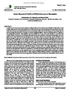
Therefore, a strategy using neighbourhood information has been proposed and exploited by Atzberger (2004). In this “patch-ensemble” or “object-based” approach the covariances between spectral variables over a certain number of pixels representing the same class of object (e.g., an agricultural field) are analysed. The method requires therefore remotely sensed imagery with a spatial resolution sufficient enough to distinguish the different objects (such as provided by the future Sentinel-2 sensor). Relying on synthetic data, Atzberger (2004) demonstrated that the “object signature” contains valuable additional information to mitigate the compensation between LAI and the average leaf angle (ALA) in the inversion process. Positive effects of neighbourhood information and/or the use of per-field signatures are well known for land use and land cover classifications (Blaschke, 2010; Cremers et al., 2007; Guerif et al., 1996). The main objective of the present study is to demonstrate the effectiveness of the object-based RTM inversion for the Sentinel-2 band setting and GSD using spectral data acquired by CHRIS/PROBA. The effectiveness of the proposed approach is assessed: (i) against reference LAI measurements (Barrax campaign), (ii) with respect to the spatial consistency of the retrieved biophysical fields, and (iii) through comparison of retrieval accuracies with those obtained from a standard RTM inversion approach and a simple empirical method using the Normalized Difference Vegetation Index (NDVI). The study is an extension of a previously published conference paper based on the same test data set (Atzberger and Richter, 2009). It further extends the original idea developed on synthetic data (Atzberger, 2004) and provides graphical illustrations of the underlying concept. 2. Materials and methods 2.1. Experimental site and observations For the application of the proposed inversion technique, observations of the interdisciplinary ESA SPARC 2004 campaign (Moreno et al., 2004) were used. The field campaign was carried out in July 2004 at the Barrax site (N 30° 3′, W 2° 6′), an agricultural test area situated in the Castilla–La Mancha region, in southern Spain. Different satellite and airborne data were obtained concurrently with measurements of vegetation parameters for a range of crops, including alfalfa, maize, potatoes, sunflower, garlic and sugar beet. The crops were grown on large uniform land use units (Fig. 1), offering an ideal data basis for the study objectives. Experiencing with the same data set, it was noticed through forward modelling that the PROSAIL radiative transfer model is not well

Fig. 1. Study area Barrax during the SPARC 2004 field campaign: CHRIS/PROBA image of 16 July 2004 at 11:25 UTC with the positions of LAI ground observations (black dots). The study mainly relies on the three fields with blue field boundaries. Results for three additional crops (in yellow) are presented in less detail.

Author's personal copy 210

C. Atzberger, K. Richter / Remote Sensing of Environment 120 (2012) 208–218

representing the spectral behaviour of row crops such as maize, potatoes and sunflower (see also Section 2.5). For this reason results will be presented separately for alfalfa, garlic and sugar beet (well simulated in forward mode) and maize, potatoes and sunflower (where the forward simulation indicated model limits). 2.1.1. EO data acquisition Hyperspectral and multi-angular data from CHRIS instrument (Compact High Resolution Imaging Spectrometer) on the PROBA platform (Project for On-Board Autonomy), were acquired over the Barrax site on 16 July 2004 at 11:25 UTC. Geometric and atmospheric corrections of the CHRIS data were performed by the Department of Thermodynamics of the University of Valencia, Spain (Guanter et al., 2005). The authors applied a dedicated atmospheric correction algorithm together with radiometric calibration of the data in an autonomous process, without the need for ancillary data (Vuolo et al., 2008). For the retrieval of top-of-canopy (TOC) reflectances the approach relies on scene-extracted reference spectra. For the purpose of the present study, only the imagery with the viewing angle closest to nadir (i.e., 8.4°) was considered. CHRIS data were acquired in Mode-1 with 62 spectral bands (from 400 nm to 1050 nm) and a spatial resolution of 34 m. For the present study, we selected a multi-spectral data set closely matching the future Sentinel-2 sensors data (Martimort et al., 2007), which involved the following CHRIS wavebands: 492, 563, 664, 706, 738, 773, 844 and 862 nm (corresponding to Sentinel-2: 490, 560, 665, 705, 740, 775, 842 and 865 nm, Drusch et al., 2010). In this way, the main spectral bands of Sentinel-2 with the purpose to retrieve LAI and other vegetation characteristics were included (Drusch et al., 2010). However, as the CHRIS data does not include SWIR bands, these could not be simulated for the upcoming Sentinel-2 sensor. It was also not possible to take into account the better spatial resolution of Sentinel-2 as compared to CHRIS data. Hence, any results reported in this study with respect to future Sentinel-2 performance must remain preliminary. However, as Sentinel-2 will have a better spectral and ground sampling compared to the current simulation, it is expected that the proposed RTM inversion will benefit. 2.1.2. Field measurements Ground-based observations of LAI were collected with the Plant Canopy Analyzer LAI-2000 instrument (LI-COR Inc., Lincoln, NE, USA). Each LAI value was the result of an average of 24 measurements taken randomly within a circular Elementary Sampling Unit (ESU) of approximately 15 m radius. No corrections were performed to account for clumping or the influence of non-photosynthetic plant components (such as stems or wilted leaves). Therefore, the term ‘LAI’ used in this paper must be understood as ‘effective plant area index’ (PAIeff) (Chen et al., 1997; Neumann et al., 1989; Richter et al., 2011). A data set of 26 LAI measurements situated within the area covered by the CHRIS imagery (Fig. 1) was selected for detailed analysis: alfalfa (5 ESUs), sugar beet (9 ESUs) and garlic (12 ESUs). At the time of the field measurement campaign, these crops showed a homogeneous coverage with evenly plagiophile (sugar beet, alfalfa) or erectophile (garlic) leaf angle distributions. Following an independent sampling strategy, leaf chlorophyll content (i.e. chlorophyll a + b) measurements were performed within the three fields for which LAI was measured: alfalfa (1 ESU), sugar beet (1 ESU) and garlic (4 ESUs). Within each ESU, roughly 50 measurements with the CCM-200 Chlorophyll Content Meter were performed. Largest leaves were chosen since the CCM-200 instrument is designed to work with leaves >1 cm of diameter. In order to enable measurements of thick and cylindrical shaped leaves of garlic, leaves scissors were used to split different layers. As far as possible, leaf veins were avoided that may perturb the measurement. Once the leaf was inside the CCM-200 window, three straight measurements were made in the same part of

the leaf. When measurement dispersion observed for an ESU was large, measurements continued until dispersion decreased sufficiently. From the leaf fraction measured with the chlorophyll-meter two samples were extracted for the posterior instrument calibration in the laboratory. They were cut by means of a copper cylinder with a sharp edge, leading to a sample with an area of (0.785 ± 0.016) cm2. These samples were located inside a previously numerated aluminium foil to keep them, and were preserved in liquid Nitrogen. Ten leaf samples were collected per field to allow calibration of the chlorophyll-meter readings using standard laboratory procedures (SPARC Data Acquisition Report, 18307/04/NL/FF). Table 1 depicts the main biophysical characteristics of the three intensively studied crops from the SPARC 2004 field campaign measurements, including the results for LAI and leaf chlorophyll content. Moreover, the table lists the same information for the three crops where forward simulations with PROSAIL indicated RTM limitations (i.e. potatoes, sunflower and maize). 2.2. Radiative transfer modelling The combined leaf (‘PROSPECT’) and canopy (‘SAIL’) reflectance model (‘PROSAIL’) was selected for this study (Jacquemoud and Baret, 1990; Kuusk, 1991; Verhoef, 1984). This model, widely validated and applied for reflectance modelling studies (e.g., Darvishzadeh et al., 2008b; Jacquemoud et al., 2009; Richter et al., 2009; Weiss et al., 2000), presents a good compromise between the complexity of the processes, accuracy and computation time requirements. The top-of-canopy (TOC) reflectance is simulated by the SAIL model as a function of three canopy structural variables, including LAI (m 2/m 2), ALA (deg; assuming an ellipsoidal distribution), and the hot spot parameter, Hot (m/m). As additional inputs the model requires the fraction of diffuse incoming solar radiation (skyl) and the view and illumination geometry (i.e. sun zenith angle, θs (deg); sensor viewing angle, θo (deg) and azimuth angle between sun and sensor, ϕ (deg)). Leaf hemispherical reflectance and transmittance are simulated by PROSPECT as a function of four structural and biochemical leaf parameters: leaf chlorophyll a + b concentration, Cab (μg/cm 2); leaf dry matter content, Cm (g/cm 2); leaf water thickness, Cw (cm) and a leaf mesophyll structural parameter, N (unitless). To obtain a representative background reflectance, the average soil signature was calculated from bare soil pixels identified in the imagery and inserted into the model. Using a (multiplicative) scaling factor, αsoil, changes in soil brightness were taken into account. Changes in soil brightness result from variations of soil moisture or surface roughness and may strongly influence the canopy reflectance (Darvishzadeh et al., 2008c). The soil background is most influential for low vegetation coverage or erectophile canopies (Atzberger et al., 2010; Bach and Verhoef, 2003).With respect to the fraction of diffuse incoming solar radiation (skyl), a fixed value of 0.1 across all

Table 1 Biophysical characteristics (mean ± standard deviations) of the crops sampled during the SPARC 2004 field campaign: LAI, total above ground dry matter, mean tilt angle (MTA) and leaf chlorophyll content. Note that the number of sampled elementary sampling units (ESU) for LAI measurements is different from the number of ESUs for leaf chlorophyll.

Alfalfa Sugar beet Garlic Potatoesa Sunflowera Maizea

ESU

LAI

Dry matter

(LAI)

m2/m2

g/m2

5 9 12 15 6 11

3.7 ± 0.7 4.9 ± 0.5 0.7 ± 0.1 4.9 ± 1.0 0.6 ± 0.1 2.4 ± 0.6

90 ± 20 72 ± 11 130 ± 30 43 ± 3 – 61 ± 6

MTA

ESU (Cab)

53 ± 8 42 ± 1 64 ± 8 41 ± 5 47 ± 10 50 ± 4

2 1 4 2 4 3

Chlorophyll content μg/cm2 49.3 ± 0.7 48.9 ± 0.62 49.2 ± 2 36.5 ± 0.7 42.7 ± 0.5 51.6 ± 0.8

a Not intensively studied, as forward simulations with PROSAIL revealed RTM limitations.


211

wavelengths was used, as in many similar studies (Richter et al., 2011). Hence, we have neglected the fact that the amount (and spectral distribution) of diffuse sky light depends on atmospheric conditions, solar zenith angle, and wavelength. This simplification seems justified, however, by the fact that skyl has only a very small influence on canopy reflectance (Clevers and Verhoef, 1991; Yao et al., 2008) and by the lack of on-site measurements of skyl.

were chosen, closely matching the configuration of the future ESA satellite Sentinel-2 (Martimort et al., 2007) (see also Section 2.1). This spectral sampling was tested for its suitability for LAI estimation by Richter et al. (2009).

2.3. Look-up-table (LUT) generation for RTM inversion

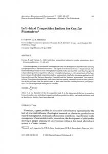
In the case of the pixel-based LUT inversion (LUTpix), the solution of the inverse problem is selected by applying a simple cost function calculating the root mean square error (RMSE) pixel-wise between simulated and measured spectra (e.g., Darvishzadeh et al., 2008b). The solution consists in the PROSAIL parameter combination yielding the lowest RMSE. No attempts were made to evaluate the usefulness of using the average of multiple solutions or other regularisation strategies proposed in the literature. The regularization with the object-based RTM inversion (LUTobj) explicitly consisted in considering the spatial dependency between the pixels. For this purpose, a two-step LUT approach was used aiming to determine one optimum ALA value for all pixels of a given agricultural object. In Fig. 2 the working flow is illustrated. A graphical illustration of the object-based inversion is given in Fig. 3. The object-based inversion assumes that ALA is constant inside a given agricultural field (Atzberger, 2004). Within a gliding 3 × 3 pixel window, it is further hypothesized that the main spectral variation is due to changes in LAI, whereas variations in Cab, Cm, Hot and soil brightness (Θ) can be neglected (Fig. 3D). In the current implementation, the simulations are performed separately for each of the eleven ALA values (from 20° to 70°) by selecting each time the solution that minimizes the RMSE of all nine signatures within the 3 × 3 window. This is done by calculating for each of the 1.000 Θ combinations the overall RMSE for the nine pixels, allowing only LAI to vary from pixel to pixel. For each ALA value, solely the parameter combination with the lowest overall RMSE is kept. This yields for the central pixel within the gliding window (and for each ALA value) the retrieved candidate solutions (Θ × LAI) and the associated cost function values (RMSE). Advantage is therefore taken of the geostatistical principle that nearby pixels are more similar than pixels further apart and that the model parameters – in most cases – vary only smoothly in space (Curran and Atkinson, 1998). At the same time spectral neighbourhood information is taken into account. As for each of the eleven candidate solutions (one for each ALA) information on the goodness of fit is available, this first step already allows in principle to map the RTM parameters in a spatially consistent way (albeit ALA is not yet optimized to a unique value across the whole image object). The simultaneous (and constrained) inversion of the first step assumes that the pixels within a gliding window are situated on “soil

A LUT based inversion method is chosen for the present study, since it is easy to implement while providing robust and accurate RTM inversions (Richter et al., 2009, 2011; Weiss et al., 2000). For comparison purposes, the proposed object-based RTM inversion (‘LUTobj‘) is supplemented by a pixel-based inversion approach (‘LUTpix‘). To ensure that the results of the two procedures are fully comparable, the same basic LUT is used. The sole difference consists in the way the spectral information is presented to the LUT. This will be further detailed in Section 2.4. To generate a synthetic LUT data base, the PROSAIL model was run in forward mode to simulate bidirectional canopy reflectances (400 to 2500 nm) for a defined number of canopy realizations. A relatively large LUT size of 1.056.000 parameter combinations was chosen without using any a priori information from the campaign measurements. The RTM variables were either sampled randomly within uniform distributions (Cab, Cm, αsoil, Hot) or in regular steps (ALA). LAI, being the variable of most interest, was drawn within an asymmetric distribution from 0 ≤ LAI ≤ 8. In order to account for the strong sensitivity of the canopy reflectance to LAI for small LAI values, the distribution was positively skewed giving most emphasis on LAI values b 1 (Asner et al., 2003; Baret et al., 2007). The second Pearson's skewness coefficient (Sk) for this distribution resulted in a value of Sk = 0.198. To account for a possibly large range of leaf orientations, ALA was sampled in 11 regular steps from 20° ≤ ALA ≤ 70°. The range of Cab was set between 20 and 70 μg/cm 2 to cover its plausible range (Table 1). Cw was fixed to an arbitrary value (0.02) because the absorption of leaf water does not influence significantly the canopy reflectance in the spectral range used (b0.9 μm). The leaf structure parameter N was fixed to a reasonable value (N = 2.0) (e.g. Vuolo et al., 2008). The parameter skyl was set to 0.1 across all wavebands, according to similar studies (Richter et al., 2009), and taking its limited impact on canopy reflectance into account (Clevers and Verhoef, 1991; Yao et al., 2008). Illumination and viewing conditions corresponded to the situation of the satellite overpass: θs = 21°, θο = 8.4° and ϕ = 138°. The bounds and distributions of the various RTM parameters are given in Table 2. To minimize redundancy of spectral data (Price, 1994) and to speed up the calculation process of the LUT, only 8 out of the 62 CHRIS bands

2.4. Spatially constrained regularization strategy and pixel-based inversion

Table 2 Number, ranges, mean and distribution of the input variables for the PROSAIL radiative transfer model for the generation of the LUT database. In a first step, 1000 combinations of [Cab × Cm × Hot × αsoil ], called Θ, were randomly drawn within the specified bounds. These combinations were then systematically crossed with the 96 LAI values and the 11 average leaf angles (ALA). Parameter LAI ALA Hot Cab Cm αsoil Cw N skyl θs θο ϕ

Number

Θ

96 11 1000

1 1 1 1 1 1

Min 0.001 20 0.01 20 0.004 0.6 n.a. n.a. n.a. n.a. n.a. n.a.

Mean 3.4 45 0.49 45 0.0055 1.0 0.02 2.0 0.1 21 8.4 138

Max 8.0 70 1.0 70 0.007 1.4 n.a. n.a. n.a. n.a. n.a. n.a.

Units 2

Distribution 2

m /m deg m/m μg/cm2 g/cm2 unitless cm unitless fraction deg deg deg

Asymmetric (positive skew) Regular Uniform

Fixed Fixed Fixed Fixed Fixed Fixed



Fig. 2. Illustration of the working flow for object-based and pixel-based RTM inversion.

trajectories” or “soil isolines” (Shabanov et al., 2002) in the 8dimensional feature space (Fig. 3A). The various subplots of Fig. 3 illustrate the underlying principle of the object based RTM inversion in the 2-dimensional (Red and nIR) feature space (with Cab, Cm and Hot fixed). For illustration purposes the hypothetical location of 3 × 3 pixels is shown as well (Fig. 3D). As for a given ALA different Θ will yield different “soil trajectories”, this first step optimizes Θ. One goodnessof-fit value per ALA value (and per window position) is thus obtained. To select the optimum ALA value for all pixels of a given image object, a second step is required, in which solely the candidate solutions of the first step are considered (Θ × LAI). The sum of the individual goodness of fit values (RMSE) across all pixels within a given crop field (i.e., image object) is calculated per ALA value. In the implemented algorithm, the object-wise optimized ALA value is the one yielding the lowest sum of RMSE values. Taking into account that a given image object (agricultural field) is cropped with the same species in a similar development stage (hence all pixels should have more or less the same ALA), the counterbalancing

effects between ALA, respectively αsoil, and LAI are thus effectively reduced without the need of prior information concerning ALA or αsoil. The object-based inversion also ensures a certain spatial smoothness of the retrieved RTM parameters as the errors between measured and simulated spectral signatures are not driven to ever smaller values without taking care of spatial consistency. On the contrary, as a “soil trajectory” has to fit all pixels within a (gliding) window (Fig. 3D), the retrieved parameter fields are necessarily smooth. The smoothness of the retrieved parameters increases further once the second step (ALA optimization) has been accomplished. 2.5. Suitability of PROSAIL for selected crops assessed through forward modelling A prerequisite of model inversion is the capability of the RTM to simulate properly the canopy spectra of the crops studied (Baret and Buis, 2008). Hence, the suitability of the PROSAIL model was evaluated, quantifying the agreement between measured and simulated


213

or high discrepancies between measured and simulated spectra) and to present/discuss the results accordingly. 2.6. Scaled NDVI as baseline comparison To demonstrate the validity of the physically based approaches over empirical methods, the ‘scaled NDVI’ was additionally applied for LAI estimation. The scaled NDVI approach is a method commonly used for spatial variable retrieval for two-source energy balance (TSEB) modelling (Choudhury et al., 1994; Richter and Timmermans, 2009). Hereby, fraction of vegetation cover (fCover) is first determined from NDVI. The equation is composed of end-member NDVI values, characterizing surfaces fully covered and completely uncovered by vegetation, respectively. LAI is then calculated from fCover by means of a logarithmic function (for equation and further details see Richter and Timmermans, 2009). 3. Results and discussions 3.1. Plausibility of the retrieved parameter distributions

Fig. 3. Principle of the ill-posed inverse problem and the object-based RTM inversion illustrated in the red-nIR feature space using PROSAIL simulations. For all simulations constant leaf optical properties are assumed: Cab = 50; Cm = 0.01; Hot= 0.25. [A] spectral trajectory (“soil trajectory”) obtained for one leaf angle (ALA) and one soil brightness (αsoil), when LAI varies between 0 and 10, [B] “soil trajectories” for 5 soil brightness values and three ALA, [C] ill-posed inverse problem: different combinations of ALA× αsoil yield an identical crossing point, [D] object-based RTM inversion; only one “soil trajectory” fits all nine pixels within a gliding (3× 3) window. The black dots (plus the rectangle = central pixel) represent the hypothetical position of nine pixels within a 3 × 3 (gliding) window. Assuming that over short distances (± 1 pixel) variations in soil brightness can be neglected, the proposed object-based inversion searches for one common set of ALA × αsoil so that the resulting “soil trajectory” best fits the nine measured pixels.

signatures using field measured biophysical variables as input. For each plot (ESU) an individual training database (LUT) was established. For the LUTs 10,000 variable combinations were created. Variables were randomly sampled using ESU-specific measurements of LAI and field-specific measurements of ALA and Cab. To take into account possible measurement errors, the measured values for these three variables (+soil brightness) were varied, i.e., LAI with factors 0.8 and 1.2, Cab and αsoil with factors 0.7 and 1.3, and ALA was set ±15° compared to the ground information (Table 1). The other variables were varied according to Table 2. The reflectance mismatch was defined with the minimum RMSE, calculated between the measured spectrum and the best fitting spectrum of the plot-specific LUT. The procedure was repeated for all ESUs of all crops (58) to verify that PROSAIL does indeed well simulate the observed canopy signatures. Calculating the average RMSE of the two worst ESUs of each crop, results revealed that garlic performed best (RMSE: 0.0078), followed by sugar beet (RMSE: 0.0133) and alfalfa (RMSE: 0.0150). The three remaining crops were simulated with lower accuracies: maize (RMSE: 0.0163), potatoes (RMSE: 0.0174) and sunflower (RMSE: 0.0185); probably as a result of (strong) row effects not taken into account by the 1D PROSAIL model. Strong row effects were for example evident during the actual growth stages of sunflower and maize. Similar findings were revealed by Richter et al. (2009). In the case of potatoes, the reason may be found in the deep soil groves partly filled with water due to special agronomic soil practises (Vuolo et al., 2008). Such a peculiarity is, however, difficult to take into account by simple models such as PROSAIL using a simple soil factor to simulate reflectance variations caused by soil moisture. This issue needs, however, further detailed investigation. Hence, for the present study, we decided separating the six crops into two groups (i.e. low

The PROSAIL radiative transfer model was inverted over data emulating the future Sentinel-2 sensors using LUTpix, the pixel-wise LUT approach and LUTobj, where the RTM inversion was performed in 3 × 3 gliding windows. The resulting spatial patterns of the retrieved variables show similar patterns for both methods. The object-based approach, however, obtained smoother spatial distributions compared to the pixel-based inversion. The increased smoothness and spatial autocorrelation is graphically illustrated in Fig. 4 in the form of maps and transects of the retrieved soil brightness factor (αsoil) for the alfalfa field. (Similar results are found for the other PROSAIL parameters and crops, but not shown). In view of the uniform irrigation by centre pivot systems, high gradients as presented in the “pixel-based field” (Fig. 4, left) are rather unrealistic. Moreover, in the “object-based field” (Fig. 4, right) there are low αsoil values along the pivot (from lower left to upper right), implying highest soil moisture. This may better depict the actual situation with pivot sprinklers watering the adjacent area than the high variability of αsoil found by the pixelbased approach. The retrieved parameter distributions for the three ‘suitable’ and three ‘less suitable’ crops are summarized in Table 3 for the proposed inversion algorithm (LUTobj). For each retrieved PROSAIL parameter

Fig. 4. Influence of the proposed RTM regularization on the retrieved soil brightness factor (αsoil) for the alfalfa test field. The soil brightness factor is shown as maps (top) and in the form of a spatial transect through the centre of the pivot field. The comparison is between the pixel-based inversion approach (left map and red line) and the proposed regularization based on the neighbourhood information (right map and blue line). The NDVI image is only added for illustration purposes.



Table 3 Modelled PROSAIL variables at field level using the object-based and pixel-based RTM inversions (LUTobj and LUTpix, respectively). For each crop, the intra-field average is indicated (μ) as well as the coefficient of variation (CV). The table distinguishes between ‘suitable’ crops (with good forward simulation results) and ‘less suitable’ crops (were the forward modelling indicated relatively large deviances between measured and simulated canopy spectra). LAI

Alfalfa Sugar beet Garlic Potatoa Sun-flowera Maizea a

μ CV μ CV μ CV μ CV μ CV μ CV

Cab

Cm

ALA

αsoil

Hot

LUTobj

LUTpix

LUTobj

LUTpix

LUTobj

LUTpix

LUTobj

LUTpix

LUTobj

LUTpix

LUTobj

LUTpix

3.63 0.13 3.41 0.33 0.62 0.29 2.27 0.36 1.68 0.32 4.61 0.27

2.46 0.13 2.23 0.28 0.51 0.47 1.78 0.33 1.08 0.52 3.63 0.22

61.5 0.02 59.7 0.03 44.5 0.04 44.8 0.07 46.8 0.04 57.1 0.04

68.4 0.02 67.8 0.03 45.2 0.22 42.9 0.16 57.0 0.15 63.9 0.07

0.0055 0.01 0.0055 0.01 0.0056 0.01 0.0056 0.01 0.0056 0.01 0.0056 0.01

0.0044 0.15 0.0045 0.15 0.0056 0.13 0.0053 0.15 0.0051 0.14 0.0049 0.15

45 n.a. 50 n.a. 70 n.a. 45 n.a. 70 n.a. 70 n.a.

22 0.19 29 0.46 60 0.25 28 0.45 53 0.26 67 0.05

0.24 0.34 0.47 0.13 0.51 0.03 0.43 0.21 0.47 0.10 0.37 0.24

0.08 0.70 0.20 1.22 0.50 0.57 0.12 1.39 0.23 1.07 0.21 0.95

0.89 0.04 0.90 0.06 0.87 0.07 0.82 0.08 0.70 0.06 0.78 0.08

0.81 0.15 0.86 0.18 0.85 0.07 0.88 0.15 0.63 0.06 0.81 0.20

Not intensively studied, as forward simulations with PROSAIL revealed RTM limitations.

the average (μ), as well as the coefficient of variation (CV), are indicated. Both descriptive statistics refer to all pixels within the respective field. The CV was included to characterize the modelled intra-field variability. For comparison, the results of the standard inversion approach (LUTpix) are also specified. Cumulative distribution functions resulting from the two inversion approaches are shown in Fig. 5 for the three ‘suitable’ crops. As identical LUTs were used in both cases, any differences between pixel- and object-based approaches are solely the result of using (or not) the neighbourhood information. The comparison of LAIobj and LAIpix in Table 3 emphasizes the impact of the proposed algorithm. The regularization strongly reduces the intra-field variability of PROSAIL parameters compared to the pixelbased inversion approach. The high CV of many of the PROSAIL parameters in the pixel-based inversion is a direct result of the ill-posed inverse problem. Indeed, through selection of (extreme) parameter combinations, the error between modelled and observed spectral signature is driven to very small values. This, however, comes at the cost of implausible high CV of the pixel-based RTM inversion. It also results in

a lack of spatial autocorrelation of the retrieved parameters, as shown exemplarily for the retrieved soil brightness of the alfalfa field (Fig. 4). This lack of spatial consistency and realism of the simulations is effectively reduced by LUTobj as the proposed regularization analyzes the spectral information within 3 × 3 gliding windows. As illustrated in Fig. 3D, the spectral information within the 3 × 3 gliding window has to be fitted by a single parameter setting [Θ × LAI × ALA], leading to an object-based inversion and smoother parameter fields. These findings can be further discussed for the alfalfa test field (Fig. 5; top row). Ignoring the neighbourhood information, there is a clear tendency of the LUTpix approach to select extreme parameter combinations. The LUTpix retrieved ALA values are predominantly at the lower bound (ALA= 20), whereas very high leaf chlorophyll concentrations are modelled (Cab) together with small hot spot values (Hot). The intra-field variations in soil brightness (αsoil) and leaf dry matter content (Cm) are extremely large. Altogether this yields spatially inconsistent and implausible parameter fields for alfalfa. The (positive) impact of the proposed object-based inversion on the retrieved ALA

Fig. 5. Retrieved intra-field PROSAIL parameter distributions in the form of cumulated distribution functions (blue: proposed algorithm; red: standard inversion approach). The limits (minimum and maximum) of the x-axes correspond to the ranges of the LUT. The number of pixels per field (n) are also indicated.


values for the alfalfa field is visible in Fig. 5 (top row; blue line). After the first step of the inversion approach (not shown), the retrieved leaf angles remain mostly in the range of 40–50°. With the second step of the LUT inversion, an optimum value of ALA of 45° representative for the entire alfalfa field is found. Both optimization steps yield on one hand higher estimated LAI values compared to LUTpix. At the same time, all other PROSAIL parameters remain within relatively small (and plausible) ranges. Apparently, for each pixel in the alfalfa field, there is at least one set of [Θ × LAI] for low ALA that fits the individual spectra very well, and with lower RMSE as compared to [Θ × LAI] for higher ALA values. However, there seems to be no [Θ × LAI] combination for low ALA fitting concurrently all signatures within a 3 × 3 window. Hence, higher ALA values are selected for LUTobj. Similar interpretations apply for the sugar beet and garlic fields. Though field measurements are not available to assess the estimation accuracy of the individual PROSAIL parameters (except LAI and Cab) it can be safely stated that coefficients of variations as shown in Table 3 and Fig. 5 for the standard (pixel-based) inversion are highly unrealistic. This is first, because the fields are grown with genetically identical plant material under homogeneous management conditions (e.g. sowing date), and second, because all plants in a given field are in a very similar development stage. The situation changes dramatically, once the spatial information is taken into account. The retrieved fields are smooth with intra-field variabilities reduced to plausible ranges.

3.2. Retrieved LAI values and comparison with field measurements Scatter plots between observed and retrieved LAI values are shown in Fig. 6 for the three ‘suitable’ crops and the two inversion approaches. The corresponding error statistics calculated between the modelled LAI and the SPARC field measurements are specified in Table 4 for each of the three ‘suitable’ crops, as well as for the three crops where forward simulations revealed RTM limitations. The average difference (Δμ) and the root mean square error (RMSE) between observations and estimates are indicated, as well as the corresponding number of independent observations (ESUs) used for the assessment. Fig. 6 and the results summarized in Table 4 clearly demonstrate the added value of the spectral neighbourhood information for regularizing the ill-posed inverse problem. For the ‘suitable crops, the retrieved LAI values show significantly decreased RMSE as compared to the pixel-based RTM inversion. For the alfalfa crop and the sugar beet field, the RMSE decreases by 55% and 66%, respectively, when spatial information is used for RTM regularization. At the same time, the observed bias (offset) is reduced by 1.2 (alfalfa) to 1.5 LAI units (sugar beet). The effect is much less pronounced for garlic, as the LAI of this crop is already well modelled without spatial information. Due to the low coverage (LAIb 1) of the garlic field, LUTpix yields ALA values reasonable for the erectophile plant architecture, and consequently produces accurate LAI estimates.

215

Table 4 Accuracy of LAI retrieval for six crops from two inversion procedures and an empirical model: (left) using the proposed object-based inversion taking neighbourhood information into account, (middle) using a pixel-based inversion, neglecting neighbourhood information, (right) using the scaled NDVI approach. The statistics are derived through comparison with ground reference measurements (Table 1). The table distinguishes (top) between ‘suitable’ crops with good forward modelling results, and (bottom) ‘less suitable’ crops where the forward modelling exercise showed problems of PROSAIL in correctly simulating the observed canopy signatures. n

Alfalfa Sugar beet Garlic All ‘suitable’ Potatoesa Sunflowera Maizea

5 9 12 26 15 6 11

Object-based inversion

Pixel-based inversion

NDVI

Δμ

RMSE

Δμ

RMSE

Δμ

RMSE

0.05 0.67 − 0.07 0.21 1.60 − 1.05 − 2.22

0.63 0.76 0.20 0.54 1.87 1.16 2.31

1.25 2.22 0.05 1.03 2.39 − 0.37 − 1.29

1.39 2.24 0.25 1.46 2.57 0.70 1.43

− 0.65 1.01 0.13 0.27 1.08 − 0.68 − 0.75

1.04 1.26 0.20 0.90 1.45 0.81 0.9

a Not intensively studied, as forward simulations with PROSAIL revealed RTM limitations.

The improved LAI retrieval accuracy for the alfalfa and sugar beet fields is a direct result of the better estimation of the average leaf angle (ALA) when using the object-based inversion. Ignoring the neighbourhood information, the retrieved ALA values for the alfalfa and sugar beet fields (Table 3) are much lower than the observed MTA (Table 1). The underestimated ALA has to be compensated by lower than observed LAI (Table 4) and high pigment concentrations, respectively, low soil brightness. Using the spatially constrained RTM inversion leads to ALA values (Table 3) which seem more reasonable with respect to the overall appearance of the crops. At the same time the retrieved ALA values come relatively close to the LAI2000 derived mean tilt angle (MTA) (Table 1), albeit the comparison of both measures (i.e. ALA and MTA) should be carried out carefully, keeping in mind the limitations of used instruments and models (see also Section 2.1). The ALA being more accurately modelled, the LAI values are also better retrieved (Fig. 6). The differences in retrieved ALA values yield on average (looking at all pixels within a given field) higher vegetation densities for the objectbased approach compared to the pixel-based approach, and a higher dynamic range (Fig. 7). Despite the large discrepancies in the retrieved distributions of variables such as αsoil, Cab and Cm, the overall correlation between LAI distributions from pixel- and object-based approaches remains quite linear. This supports again the hypothesis that the main counterbalancing effects are between LAI and ALA, with the soil brightness adding the necessary degree of freedom. The remaining biophysical variables play in this respect only a secondary role, allowing the pixel-based inversion to drive the residual error between observed and modelled spectrum to low values. At the same time our findings might explain the difficulties usually encountered when estimating

Fig. 6. Ground measured against retrieved LAI values for the three ‘suitable’ crops and the two inversion approaches. Left: proposed approach. Right: pixel-based inversion.



Fig. 7. Distribution of retrieved LAI values for the three ‘suitable’ crops and the two inversion approaches. Top: pixel-based vs. object-based retrievals. Bottom: Cumulated frequency distributions.

for example leaf pigmentation from remote sensing data. The linear relations depicted in Fig. 7 also show that an ex post averaging of pixel-based LAI retrievals would not reduce the observed deviances to the LAI observations. However, such an averaging would certainly increase the spatial smoothness of the retrieved fields. As stated in Atzberger (2004) and again in Section 2 (Methods), the proposed object-based inversion relies on additional information stemming from the spectral covariance in the canopy reflectances within the local neighbourhood (see Fig. 4C). To exclude the possibility that the improved retrieval accuracies are simply an artefact resulting from the increased spatial sampling support (i.e. 3 × 3 gliding windows against inversion of individual pixels), it was suggested (F. Baret, pers. communication) to test the pixel-based RTM inversion with spectral data averaged over 3 × 3 windows. Such a low pass filtering effectively reduces the sensor noise, but will eliminate any covariance related information used in the proposed algorithm. Testing this alternative approach, it was not possible to reproduce the good results obtained with the object-based inversion (except for garlic). The RMSE between field measured and retrieved LAI values for the alfalfa and sugar beet crops, for example, were far higher (1.39 and 2.63) as compared to the values reported for the proposed inversion (0.63 and 0.76) and even higher as those obtained from the pixelbased inversion (Table 4). This clearly confirms that the additional information stems from the consideration of the spatial covariance and is not an artefact of an increased sampling support (i.e. reduced noise). Evaluating the LAI retrieval performance of the scaled NDVI (Section 2.6) with the ground measured data leads for the ‘suitable’ crops to an overall RMSE of 0.9, which is significantly less accurate than the LUTobj approach but performs better than LUTpix. In Table 4 the crop-specific RMSE values are depicted. These results confirm the potential of the proposed regularization within physically based approaches compared to empirical methods and pixel-based RTM inversions. As expected, neither the object-based nor the pixel-based approach could simulate correctly the LAI of the three ‘less suitable’ crops (Table 4; bottom). For these crops already the forward modelling results revealed PROSAIL limitations. Under such conditions it is possible – but strongly disadviced – to run the inversion. For such cases, first an appropriate RTM needs to be selected.

3.3. Modelling of the leaf chlorophyll content Only few measurements are available for assessing the accuracy of the retrieved leaf chlorophyll content (Table 1). For example, only one ESU was sampled for Cab inside the alfalfa and sugar beet fields. Only for the garlic field, the situation is somewhat better as 4 ESUs were sampled (Table 1). Hence, in what follows only very broad trends can be indicated. One general finding is that the pixel-based inversion strongly overestimates the leaf chlorophyll content for alfalfa and sugar beet (compare Table 3 and Table 1). The overestimation is less pronounced when using the proposed algorithm (see Table 3), but still considerable. For garlic, the retrieved Cab distributions of both approaches (Fig. 5, last row) come on average close to the field measured average (Cab ~49 μg/cm 2). For this crop (with 4 ESUs), the proposed approach outperforms the pixel-based RTM inversion (Fig. 8). With this limited data set a RMSE of 3.98 μg/cm 2, a Δμ of 1.65 μg/cm 2 and R 2 of 0.80 is obtained, which is significantly better compared to the retrieval accuracy of the pixel-based inversion (RMSE: 7.33 μg/cm 2, Δμ: 6.70 μg/ cm 2, and R 2: 0.67).

Fig. 8. Ground measured against modelled leaf chlorophyll content (in μg/cm2) for the garlic field using two alternative RTM inversion approaches.


4. Conclusions Using ground observations from the SPARC 2004 campaign and the space-borne CHRIS/PROBA data spectrally resampled to the future Sentinel-2 sensor, the study has demonstrated that the proposed object-based RTM inversion (LUTobj) yields overall more accurate LAI estimates than the pixel-based LUT inversion (LUTpix). However, positive effects could only be demonstrated for alfalfa, sugar beet and garlic. As expected, analyzing potatoes, maize and sunflower was not successful (Atzberger and Richter, 2009). The failure can be attributed to the inappropriateness of the (1-dimensional) PROSAIL model for simulating the spectral behaviour of inhomogeneous (row) crops. Validation of retrieved leaf chlorophyll contents with field measurements showed rather limited estimation performance. However, the proposed approach yielded significantly improved results, compared to the standard inversion. Our results provide evidence that the spatially constrained RTM inversion reduces strong counterbalancing effects between various RTM parameters. This yields more plausible (i.e., relatively narrow) intra-field distributions of RTM parameters and spatially more consistent results. These improvements were possible due to the parallel inversion of all pixels within a gliding (3× 3) window, for which only one common set of RTM parameters is optimized. The resulting “soil trajectory” fitted best (in a least square sense) the nine pixels in the 8-dimensional feature space. The proposed 2-step inversion scheme can be easily adapted to different needs and the paper gives the necessary details for an effective implementation. For demonstration purposes only a simple turbid medium model (e.g. PROSAIL) was used. However, the algorithm can be employed with any kind of model, including those taking into account the 3-dimensionality of canopy architectures (Schlerf and Atzberger, 2006). 3D-models are particularly recommended for analyzing vegetation with complex canopy geometries, e.g. row-structured crops or forests. In future analyses it will be evaluated whether the objectbased inversion with such a RTM is better capable to simulate bidirectional reflectance of row planted crops. However, the application of the proposed regularization is not necessarily restricted to vegetation studies (Atzberger et al., 2004). For a possible application in operational vegetation monitoring, the implementation of the methodology requires a classification/ segmentation of the area of interest for the detection of field/object boundaries to be performed in advance of the calculations. Also, pixel sizes must be small enough to resolve individual fields. With a GSD of 10 m, the future Sentinel-2 sensor is in this respect well suited for the proposed approach. At the same time it should be insured that growing conditions are homogeneous within the detected field boundaries. It must be emphasized that the proposed regularization approach can tackle the ill-posedness at canopy level, but not a possible illposedness within the employed leaf optical properties model. Further research is required in this regard. A major advantage of the proposed algorithm is that no prior information concerning the various RTM parameters is necessary (e.g., parameter bounds). However, if available, prior information could be easily incorporated. Conclusively, for the operational analysis of the future Sentinel-2 data it is strongly recommended to implement algorithms taking neighbourhood information into account, mitigating the ill-posed inverse problem and thus leading to higher estimation accuracies.

References Asner, G. P., Scurlock, J. M. O., & Hicke, J. A. (2003). Global synthesis of leaf area index observations: implications for ecological and remote sensing studies. Global Ecology and Biogeography, 12(3), 191–205. Asrar, G. (1989). Theory and Applications of Optical Remote Sensing. Wiley Series in Remote Sensing.

217

Atzberger, C. (2004). Object-based retrieval of biophysical canopy variables using artificial neural nets and radiative transfer models. Remote Sensing of Environment, 93, 53–67. Atzberger, C. (2010). Inverting the PROSAIL canopy reflectance model with neural nets trained on streamlined data sets. Journal of Spectral Imaging, 1. doi:10.1255/ jsi.2010.a2. Atzberger, C., Baret, F., Guérif, M., & Werner, W. (2010). Comparative analysis of three chemometric techniques for the spectroradiometric assessment of canopy chlorophyll content in winter wheat. Computers and Electronics in Agriculture, 73(2), 165–173. Atzberger, C., Houlès, V., Guérif, M., Machet, J. M., & Mary, B. (2004). Site specific calibration of a crop model by assimilation of observations derived from remote sensing. Geophysical Research Abstracts, 6 EGU04-A-04353. Atzberger, C., & Richter, K. (2009). Geostatistical regularization of inverse models for the retrieval of vegetation biophysical variables. In U. Michel, & D. L. Civco (Eds.), SPIE's 2009 conference proceedings: Remote Sensing for Environmental Monitoring, GIS Applications, and Geology IX (pp. 74781O). Bach, H., & Verhoef, W. (2003). Sensitivity studies on the effect of surface soil moisture on canopy reflectance using the radiative transfer model GeoSAIL. Proceedings of IGARSS, 2003, 1679–1681. Bacour, C., Baret, F., Béal, D., Weiss, M., & Pavageau, K. (2006). Neural network estimation of LAI, fAPAR, fCover and LAI×Cab, from top of canopy MERIS reflectance data: Principles and validation. Remote Sensing of Environment, 105(4), 313–325. Baret, F., & Buis, S. (2008). Estimating canopy characteristics from remote sensing observations. In S. Liang (Ed.), Review of methods and associated problems. Advances in Land Remote Sensing: System, Modeling, Inversion and Application. (pp. 172–301) Netherlands: Springer. Baret, F., & Guyot, G. (1991). Potentials and limits of vegetation indices for LAI and APAR assessment. Remote Sensing of Environment, 35, 161–173. Baret, F., Hagolle, O., Geiger, B., Bicheron, P., & Miras, B. (2007). LAI, fAPAR and fCover CYCLOPES global products derived from VEGETATION Part 1: Principles of the algorithm. Remote Sensing of Environment, 110, 275–286. Baret, F., Jacquemoud, S., Guyot, G., & Leprieur, C. (1992). Modeled analysis of the biophysical nature of spectral shifts and comparison with information content of broad bands. Remote Sensing of Environment, 41(2–3), 133–142. Blaschke, T. (2010). Object based image analysis for remote sensing. ISPRS International Journal of Photogrammetry and Remote Sensing, 65(1), 2–16. Chen, J. M., Rich, P. M., Gower, S. T., Norman, J. M., & Plummer, S. (1997). Leaf area index of boreal forests: Theory, techniques and measurements. Journal of Geophysical Research, 102(24), 29429–29444. Cho, M., Skidmore, A., & Atzberger, C. (2008). Towards red-edge positions less sensitive to canopy biophysical parameters for leaf chlorophyll estimations using properties optique spectrales des feuilles (PROSPECT) and scattering by arbitrarily inclined leaves (SAILH) simulated data. International Journal of Remote Sensing, 29(7–8), 2241–2255. Choudhury, B. J., Ahmed, N. U., Idso, S. B., Reginato, R. J., & Daughtry, C. S. T. (1994). Relations between evaporation coefficients and vegetation indices studied by model simulations. Remote Sensing of Environment, 50, 1–17. Clevers, J. G. P. W., & van Leeuwen, H. J. C. (1996). Combined use of optical and microwave remote sensing data for crop growth monitoring. Remote Sensing of Environment, 56(1), 42–51. Clevers, J. G. P. W., & Verhoef, W. (1991). Modelling and synergetic use of optical and microwave remote sensing. Report 2: LAI estimation from canopy reflectance and WDVI: A sensitivity analysis with the SAIL model, BCRS Report 90-39, p. 70. Colombo, R., Bellingeri, D., Fasolini, D., & Marino, C. M. (2003). Retrieval of leaf area index in different vegetation types using high resolution satellite data. Remote Sensing of Environment, 86(1), 120–131. Combal, B., Baret, F., & Weiss, M. (2002). Improving canopy variables estimation from remote sensing data by exploiting ancillary information. Case study on sugar beet canopies. Agronomie, 22(2), 205–215. Combal, B., Baret, F., Weiss, M., Trubuil, A., Macé, D., & Pragnére, A. (2002). Retrieval of canopy biophysical variables from bidirectional reflectance using prior information to solve the ill-posed inverse problem. Remote Sensing of Environment, 84, 1–15. Cremers, D., Rousson, M., & Deriche, R. (2007). A review of statistical approaches to level set segmentation: Integrating color, texture, motion and shape. International Journal of Computer Vision, 72(2), 195–215. Curran, P. J., & Atkinson, P. M. (1998). Geostatistics and remote sensing. Progress in Physical Geography, 22(1), 61–78. Danson, F. M., Rowland, C. S., & Baret, F. (2003). Training a neural network with a canopy reflectance model to estimate crop leaf area index. International Journal of Remote Sensing, 24(23), 4891–4905. Darvishzadeh, R., Atzberger, C., Skidmore, A. K., & Abkar, A. A. (2009). Leaf Area Index derivation from hyperspectral vegetation indices and the red edge position. International Journal of Remote Sensing, 30, 6199–6218. Darvishzadeh, R., Skidmore, A., Atzberger, C., & van Wieren, S. (2008). Estimation of vegetation LAI from hyperspectral reflectance data: Effects of soil type and plant architecture. International Journal of Applied Earth Observation and Geoinformation, 10(3), 358–373. Darvishzadeh, R., Skidmore, A. K., Schlerf, M., & Atzberger, C. (2008). Inversion of a radiative transfer model for estimating vegetation LAI and chlorophyll in a heterogeneous grassland. Remote Sensing of Environment, 112(5), 2592–2604. Darvishzadeh, R., Skidmore, A. K., Schlerf, M., Atzberger, C., Corsi, F., & Cho, M. A. (2008). LAI and chlorophyll estimated for a heterogeneous grassland using hyperspectral measurements. ISPRS Journal of Photogrammetry and Remote Sensing, 63(4), 409–426.



Durbha, S. S., King, R. L., & Younan, N. H. (2007). Support vector machines regression for retrieval of leaf area index from multiangle imaging spectroradiometer. Remote Sensing of Environment, 107(1–2), 348–361. Dorigo, W., Richter, R., Baret, F., Bamler, R., & Wagner, W. (2009). Enhanced automated canopy characterization from hyperspectral data by a novel two step radiative transfer model inversion approach. Remote Sensing, 1(4), 1139–1170. Drusch, M., Gascon, F., & Berger, M. (2010). GMES sentinel-2 mission requirements document. European Space Agency, 1(42). Glenn, E. P., Huete, A. R., Nagler, P. L., & Nelson, S. G. (2008). Relationship between remotely-sensed vegetation indices, canopy attributes and plant physiological processes: What vegetation indices can and cannot tell us about the landscape. Sensors, 8, 2136–2160. Goel, N. S. (1989). Inversion of canopy reflectance models for estimation of biophysical parameters from reflectance data. In G. Asrar (Ed.), Theory and Applications of Optical Remote Sensing (pp. 205–251). New York: Wiley. Goel, N. S., & Thompson, R. L. (1984). Inversion of vegetation canopy reflectance models for estimating agronomic variables. IV. Total inversion of the SAIL model. Remote Sensing of Environment, 15, 237–253. Guanter, L., Alonso, L., & Moreno, J. (2005). First results from the PROBA/CHRIS hyperspectral/multiangular satellite system over land and water targets. IEEE Geoscience and Remote Sensing Letters, 2(3), 250–254. Guerif, M., Blöser, B., Atzberger, C., Clastre, P., Guinot, J. -P., & Delecolle, R. (1996). Identification de parcelles agricoles à partir de la forme de leur évolution radiométrique au cours de la saison de culture. Photo-Interprétation, 34(1), 12–22. Haboudane, D., Miller, J. R., Pattey, E., Zarco-Tejada, P. J., & Strachan, I. (2004). Hyperspectral vegetation indices and novel algorithms for predicting green LAI of crop canopies: modeling and validation in the context of precision agriculture. Remote Sensing of Environment, 90, 337–352. Houborg, R., Anderson, M., & Daughtry, C. (2009). Utility of an image-based canopy reflectance modeling tool for remote estimation of LAI and leaf chlorophyll content at the field scale. Remote Sensing of Environment, 113, 259–274. Houborg, R., Soegaard, H., & Boegh, E. (2007). Combining vegetation index and model inversion methods for the extraction of key vegetation biophysical parameters using Terra and Aqua MODIS reflectance data. Remote Sensing of Environment, 106, 39–58. Jacquemoud, S. (1993). Inversion of the PROSPECT+SAIL canopy reflectance model from AVIRIS equivalent spectra: theoretical study. Remote Sensing of Environment, 44, 281–292. Jacquemoud, S., & Baret, F. (1990). PROSPECT: A model of leaf optical properties spectra. Remote Sensing of Environment, 34, 75–91. Jacquemoud, S., & Baret, F. (1993). Estimating vegetation biophysical parameters by inversion of a reflectance model on high spectral resolution data. In C. Varlet-Grancher, R. Bonhomme, & H. Sinoquet (Eds.), Crop structure and light microclimate: Characterization and applications (pp. 339–350). Jacquemoud, S., Baret, F., Andrieu, B., Danson, F. M., & Jaggard, K. (1995). Extraction of vegetation biophysical parameters by inversion of the PROSPECT + SAIL models on sugar-beet canopy reflectance data – Application to TM And AVIRIS sensors. Remote Sensing of Environment, 52, 163–172. Jacquemoud, S., Verhoef, W., Baret, F., Bacour, C., Zarco-Tejada, P. J., Asner, G. P., et al. (2009). PROSPECT + SAIL models: A review of use for vegetation characterization. Remote Sensing of Environment, 113, 56–66. Kimes, D., Knjazikhin, Y., Privette, J. L., Abuelgasim, A., & Gao, F. (2000). Inversion methods for physically-based models. Remote Sensing Reviews, 18, 381–440. Knyazikhin, Y., Martonchik, J. V., Myneni, R. B., Diner, D. J., & Running, S. W. (1999). Synergistic algorithm for estimating vegetation canopy leaf area index and fraction of absorbed photosynthetically active radiation from MODIS and MISR data. Journal of Geophysical Research D: Atmospheres, 103(D24), 32257–32275. Kokaly, R. F., & Clark, R. N. (1999). Spectroscopic determination of leaf biochemistry using band-depth analysis of absorption features and stepwise multiple linear regression. Remote Sensing of Environment, 67, 267–287. Kuusk, A. (1991). The hot-spot effect in plant canopy reflectance. In R. B. Myneni, & J. Ross (Eds.), Photon – vegetation interactions. Applications in Optical Remote Sensing and Plant Ecology. (pp. 139–159) New York: Springer. Lauvernet, C., Baret, F., Hascoët, L., Buis, S., & Le Dimet, F. -X. (2008). Multitemporalpatch ensemble inversion of coupled surface–atmosphere radiative transfer models for land surface characterization. Remote Sensing of Environment, 112(3), 851–861.

Le Maire, G., François, C., & Dufrêne, E. (2004). Towards universal deciduous broad leaf chlorophyll indices using PROSPECT simulated database and hyperspectral reflectance measurements. Remote Sensing of Environment, 89, 1–28. Le Maire, G., François, C., Soudani, K., Berveiller, D., Pontailler, J. Y., Bréda, N., et al. (2008). Calibration and validation of hyperspectral indices for the estimation of broadleaves forest leaf chlorophyll content, leaf mass per area, leaf area index and leaf canopy biomass. Remote Sensing of Environment, 112, 3846–3864. Liang, S. (2007). Recent developments in estimating land surface biogeophysical variables from optical remote sensing. Progress in Physical Geography, 31(5), 501–516. Martimort, P., Berger, M., Curnicero, B., Del Bello, U., Fernandez, V., Gascon, F., et al. (2007). Sentinel-2 - The optical high-resolution mission for GMES operational services. ESA Bulletin-European Space Agency, 18–23. Moran, M. S., Mass, S. J., & Pinter, P. J., Jr. (1995). Combining remote sensing and modeling for estimating surface evaporation and biomass production. Remote Sensing Reviews, 12, 335–353. Moreno, J., Melia, J., & Sobrino, J. A. (2004). The SPECTRA Barrax Campaign (SPARC): Overview and first results from CHRIS data. Proceedings of 2nd CHRIS/PROBA Workshop, Frascati, Italy, ESA-ESRIN. Neumann, H. H., Den Hartog, G. D., & Shaw, R. H. (1989). Leaf-area measurements based on hemispheric photographs and leaf-litter collection in a deciduous forest during autumn leaf-fall. Agriculture and Forest Meteorology, 45, 325–345. Peddle, D. R., Johnson, R. L., Cihlar, J., & Latifovic, R. (2004). Large area forest classification and biophysical parameter estimation using the 5-Scale canopy reflectance model in Multiple-Forward-Mode. Remote Sensing of Environment, 89(2), 252–263. Price, J. (1994). How unique are spectral signatures? Remote Sensing of Environment, 49, 181–186. Richter, K., Atzberger, C., Vuolo, F., Weihs, P., & D′Urso, G. (2009). Experimental assessment of the Sentinel-2 band setting for RTM-based LAI retrieval of sugar beet and maize. Canadian Journal of Remote Sensing, 35(3), 230–247. Richter, K., & Timmermans, W. (2009). Physically based retrieval of crop characteristics for improved water use estimates. Hydrology and Earth System Sciences, 13, 663–674. Richter, K., Atzberger, C., Vuolo, F., & D'Urso, G. (2011). Evaluation of sentinel-2 spectral sampling for radiative transfer model based LAI estimation of wheat, sugar beet, and maize. IEEE Journal of Selected Topics in Applied Earth Observations in Remote Sensing, 4, 458–464. Schlerf, M., & Atzberger, C. (2006). Inversion of a forest reflectance model to estimate structural canopy variables from hyperspectral remote sensing. Remote Sensing of Environment, 100(3), 281–294. Schlerf, M., Atzberger, C., Hill, J., Buddenbaum, H., Werner, W., & Schueler, G. (2010). Retrieval of chlorophyll and nitrogen in Norway spruce, Picea abies L. Karst, using imaging spectroscopy. International Journal of Applied Earth Observation and Geoinformation, 12, 17–26. Shabanov, N. V., Liming, Z., Knyazikhin, Y., Myneni, R. B., & Tucker, C. J. (2002). Analysis of interannual changes in northern vegetation activity observed in AVHRR data from 1981 to 1994. Geoscience and Remote Sensing, IEEE Transactions, 40(1), 115–130. Tarantola, A. (2005). Inverse Problem Theory and Methods for Model Parameter Estimation. Society for Industrial and Applied Mathematics 358 pages. Verhoef, W. (1984). Light scattering by leaf layers with application to canopy reflectance modeling: The SAIL model. Remote Sensing of Environment, 16, 125–141. Vuolo, F., Dini, L., & D′Urso, G. (2008). Retrieval of Leaf Area Index from CHRIS/PROBA data: an analysis of the directional and spectral information content. International Journal of Remote Sensing, 29(17), 5063–5072. Weiss, M., & Baret, F. (1999). Evaluation of canopy biophysical variable retrieval performances from the accumulation of large swath satellite data. Remote Sensing of Environment, 70, 293–306. Weiss, M., Baret, F., Myneni, R. B., Pragnere, A., & Knyazikhin, Y. (2000). Investigation of a model inversion technique to estimate canopy biophysical variables from spectral and directional reflectance data. Agronomie, 20, 3–22. Yao, Y., Liu, Q., Liu, Q., & Li, X. (2008). LAI retrieval and uncertainty evaluations for typical row-planted crops at different growth stages. Remote Sensing of Environment, 112(1), 94–106.