Aug 19, 2016 - Abstract. Predicate intuitionistic logic is a well established fragment of dependent types. According to the Curry-Howard isomorphism proof.
Automata Theory Approach to Predicate Intuitionistic Logic Maciej Zielenkiewicz and Aleksy Schubert
arXiv:1608.05698v1 [cs.LO] 19 Aug 2016
Institute of Informatics, University of Warsaw ul. S. Banacha 2, 02–097 Warsaw, Poland [maciekz,alx]@mimuw.edu.pl
Abstract. Predicate intuitionistic logic is a well established fragment of dependent types. According to the Curry-Howard isomorphism proof construction in the logic corresponds well to synthesis of a program the type of which is a given formula. We present a model of automata that can handle proof construction in full intuitionistic first-order logic. The automata are constructed in such a way that any successful run corresponds directly to a normal proof in the logic. This makes it possible to discuss formal languages of proofs or programs, the closure properties of the automata and their connections with the traditional logical connectives.
1
Introduction
Investigations in automata theory lead to abstraction of algorithmic processes of various kinds. This enables analysis of their strength both in terms of their expressibility (i.e. answer questions on which problems can be solved with their help) and in terms of resources they consume (i.e. time or space). They also make it possible to shed a different light on the original problem (e.g. the linguistic problem of languages generated by grammars can be reduced to the analysis of pushdown automata) which makes it possible to conduct analysis that was not possible before. In addition, the automata become a particular compact data structure that can in itself, when defined formally, be subject to further computations, as finite or pushdown automata are in automata theory. Typically, design of automata requires extraction of finite control over the process of interest. This is not always immediate in λ-calculi as λ-terms can contain bound variables from an infinite set. One possibility here consist in restricting the programming language so that there is no need to introduce binders. This method was used in the work of Düdder et al [3], which was enough to synthesise λ-terms that were programs in a simple but expressive functional language. Another approach would be to restrict the program search to programs in total discharge form. In programs of this form, one needs to keep track of types of available library calls, but not of the call names themselves. This idea was explored by Takahashi et al [10] who defined context-free grammars that can be used for proof search in propositional intuitionistic logic, which is, by
Curry-Howard isomorphism, equivalent to program search in the simply typed λ-calculus. Actually, the grammars can be viewed as performing program search by means of tree automata due to known correspondence between grammars and tree automata. However, the limitation to total discharge form can be avoided with help of the technique developed by Schubert, Dekkers and Barendregt [7]. A different approach to abstract machinery behind program search process was proposed by Broda and Damas [2] who developed a formula-tree proof method. This technique provides a realisation of the proof search procedure for a particular propositional formula as a data structure, which can be further subject to algorithmic manipulation. In addition to these investigations for intuitionistic propositional logic there was a proposal to apply automata theoretic notions to proof search in firstorder logic [6]. The paper characterises a class of proofs in intuitionistic firstorder logic with so called tree automata with global equalities and disequalities (TAGED) [4]. The characterisation makes it possible to recognise proofs that are not necessarily in normal form, but is also limited to certain class of tautologies (as the emptiness problem for the automata is decidable). In this paper we propose an automata theoretical abstraction of the proving process in full intuitionistic first-order logic. Its advantages can be best expressed in terms in which implicit, but crucial, features of proof search become explicit. In our automata the following elements of the proving process are exposed. – The finite control of the proving process is made explicit. – A binary internal structure of the control is explicated where one component corresponds to a subformula of the original formula and one to the internal operations that should be done to handle the proof part relevant for the subformula. As a by-product of this formulation it becomes aparent how crucial role the subformula property plays in the proving process. – The resource that serves to represent eigenvariables that occur in the process is distinguished. This abstraction is important as the variables play crucial role in complexity results concerning the logic [9,8]. – The automata enable the possibility of getting rid of the particular syntactical form of formulas and instead work on more abstract structures. – The definition of automaton distils the basic instructions necessary to conduct the proof process, which brings into the view more elementary operations the proving process depends on. Although the work is formulated in terms of logic, it can be viewed as synthesis of programs in a restricted class of dependently typed functional programs. Organisation of the paper We fix the notation and present intuitionistic firstorder logic in Section 2. Next, we define our automata in Section 3. We summarise the account in Section 4.
2
Preliminaries
We need to fix the notation and present the basic facts about intuitionistic firstorder logic. The notation A * B is used to denote the type of partial functions
from A to B. We write dom(w) for the domain of the function w : A * B. For two partial functions w, w0 we define w ⊕ w0 = w ∪ {hx, yi ∈ w0 | x 6∈ dom(w)}. The set of all subsets of a set A is P (A). A prefix closed set of strings N∗ over N is called a carrier of a tree. A tree is a tuple hA, ≤, L, li where A is a carrier of the tree, ≤ is the prefix order on N∗ , the set L is the set of labels and l : A → L is the labelling function. Whenever the set of labels and the labelling function are clear from the context, we abbreviate the quadruple to the tuple hA, ≤i. Since the formula notation makes it easy, we sometimes use a subtree ϕ of A to actually denote a node in A at which ϕ starts. 2.1
Intuitionistic First-Order Logic
The basis for our study is the first-order intuitionistic logic (for more details see e.g. the work of Urzyczyn, [11]). We assume that we have a set of predicates P that can be used to form atomic formulae and an infinite set X1 of first-order variables, usually noted as X, Y, Z etc. with possible annotations. Each element P of P has an arity, denoted arity(P). The formulae of the system are: ϕ, ψ ::= P(X1 , . . . , Xn ) | ϕ1 ∧ ϕ2 | ϕ1 ∨ ϕ2 | ϕ1 → ϕ2 | ∀X.ϕ | ∃X.ϕ | ⊥ where P is an n-ary predicate and X, X1 , . . . , Xn ∈ X1 . We follow Prawitz and introduce negation as a notation defined ¬ϕ = ϕ → ⊥. A formula of the form P(X1 , . . . , Xn ) is called an atom. A pseudo-atom formula is a formula of one of the three forms: atom formula, a formula of the form ∃X.ϕ, or a formula of the form ϕ1 ∨ ϕ2 . We do not include parentheses in the grammar since we actually understand the formulas as abstract syntax trees instead of strings. The tree is traditionally labelled with the cases of the above mentioned grammar. We assume that for a given case in the grammar the corresponding node of the tree has as many sons as there are non-terminal symbols in the case. In addition, we use in writing traditional disambiguation conventions for ∧, ∨ and insert parentheses to further disambiguate whenever this is necessary. The connective → is understood as right-associative so that ϕ1 → ϕ2 → ϕ3 is equivalent to ϕ1 → (ϕ2 → ϕ3 ). In a formula ϕ = ϕ1 → · · · → ϕn → ϕ0 , where ϕ0 is a pseudo-atom, the formula ϕ0 is called target of ϕ. In case ϕ0 = ∃X.ϕ00 , we call it existential target of ϕ. The set of free first-order variables in a formula ϕ, written FV1 (ϕ), is – – – –
FV1 (P(X1 , . . . , Xn )) = {X1 , . . . , Xn }, FV1 (ϕ1 ∗ ϕ2 ) = FV1 (ϕ1 ) ∪ FV1 (ϕ2 ) where ∗ ∈ {∧, ∨, →}, FV1 (QX.ϕ) = FV1 (ϕ)\{X} where Q ∈ {∃, ∀}, FV1 (⊥) = ∅.
Other variables that occur in a formula are bound. Terms that differ only in renaming of bound variables are α-equivalent and we do not distinguish between them. To describe the binding structure of a formula we use a special bind operation. Let us assume that a formula ϕ has no free variables (i.e. FV1 (ϕ) = ∅) and let ψ be its subformula together with a variable X free in
ψ. We define bindϕ (ψ, X) as the subformula of ϕ that binds the free occurrences of X in ψ, i.e. the subformula ϕ0 of ϕ such that each its proper subformula ψ 00 that contains ψ as a subformula has X ∈ FV(ψ 00 ). For instance bind⊥→∃X.⊥→P (X) (P (X), X) = ∃X.⊥ → P (X).
Γ, x : ϕ ` x : ϕ
(var)
Γ ` M1 : ϕ1 Γ ` M2 : ϕ2 (∧I) Γ ` hM1 , M2 i : ϕ1 ∧ ϕ2 Γ ` M : ϕ1 ∧ ϕ2 (∧E1) Γ ` π1 M : ϕ1 Γ ` M : ϕ1 (∨I1) Γ ` in1ϕ1 ∨ϕ2 M : ϕ1 ∨ ϕ2
Γ ` M : ϕ1 ∧ ϕ2 (∧E2) Γ ` π 2 M : ϕ2 Γ ` M : ϕ2 (∨I1) Γ ` in2ϕ1 ∨ϕ2 M : ϕ1 ∨ ϕ2
Γ ` M : ϕ1 ∨ ϕ2 Γ, x : ϕ1 ` N1 : ϕ Γ, y : ϕ2 ` N2 : ϕ (∨E) Γ ` case M of [x : ϕ1 ] N1 , [y : ϕ2 ] N2 : ϕ Γ, x : ϕ1 ` M : ϕ2 (→ I) Γ ` λx : ϕ1 .M : ϕ1 → ϕ2 Γ `M :ϕ (∀I)∗ Γ ` λXM : ∀X.ϕ Γ ` M : ϕ[X := Y ] (∃I) Γ ` pack M, Y to ∃X. ϕ : ∃X.ϕ
Γ ` M1 : ϕ1 → ϕ2 Γ ` M2 : ϕ1 (→ E) Γ ` M1 M2 : ϕ2 Γ ` M : ∀X.ϕ (∀E)∗ Γ ` M Y : ϕ[X := Y ] Γ ` M1 : ∃X.ϕ Γ, x : ϕ ` M2 : ψ (∃E)∗ Γ ` let x : ϕ be M1 : ∃X.ϕ in M2 : ψ
Γ `M :⊥ (⊥E) Γ `⊥ ⊥ϕ M : ϕ ∗
Under the eigenvariable condition X 6∈ F V (Γ, ψ). Fig. 1. The rules of the intuitionistic first-order logic
For the definition of proof terms we assume that there is an infinite set of proof term variables Xp , usually noted as x, y, z etc. with possible annotations. These can be used to form the following terms. M, N ::= x | hM1 , M2 i | π1 M | π2 M | in1ϕ1 ∨ϕ2 M | in2ϕ1 ∨ϕ2 M | case M of [x : ϕ1 ] N1 , [y : ϕ2 ] N2 | λx : ϕ.M | M1 M2 | λXM | M X | pack M, Y to ∃X. ϕ | let x : ϕ be M1 : ∃X.ϕ in M2 | ⊥ ⊥ϕ M where x is a proof term variable, ϕ, ϕ1 , ϕ2 are first-order formulas and X, Y are first-order variables. Due to Curry-Howard isomorphism the proof terms can serve as programs in a functional programming language. Their operational semantics is given in terms of reductions. Their full exposition can be found in
the work of de Groote [5]. We omit it here, but give an intuitive account of the meaning of the terms. In particular, hM1 , M2 i represents the product aggregation construct and πi M for i = 1, 2 decomposition of the aggregation by means of projections. The terms in1ϕ1 ∨ϕ2 M , in2ϕ1 ∨ϕ2 M reinterpret the value of M as one in type ϕ1 ∨ ϕ2 . At the same time case M of [x : ϕ1 ] N1 , [y : ϕ2 ] N2 construct offers the possibility to make case analysis of a value in an ∨-type. This construct is available in functional programming languages in a more general form of algebraic types. The terms λx : ϕ.M , M1 M2 represent traditional function abstraction and application. The proof terms that represent universal quantifier manipulation make it possible to parametrise type with a particular value λXM and use the parametrised term for a particular case M X. At last pack M, Y to ∃X. ϕ makes it possible to hide behind a variable X an actual realisation of a construction that uses another individual variable Y . The abstraction obtained in this way can be used using let x : ϕ be M1 : ∃X.ϕ in M2 . At last the term ⊥ ⊥ϕ M corresponds to the break instruction. The environments (Γ, ∆ etc. with possible annotations) in the proving system are finite sets of pairs x : ψ that assign formulas to proof variables. We write Γ ` M : A to express that the judgement is indeed derivable. The inference rules of the logic are presented in Fig. 1. We have now two kinds of free variables, namely free proof term variables and free first-order variables. The set of free term variables is defined inductively as follows – FV(x) = {x}, – FV(hM1 , M2 i) = FV(M1 M2 ) = FV(M1 ) ∪ FV(M2 ), – FV(π1 M ) = FV(π2 M ) = FV(in1ϕ1 ∨ϕ2 M ) = FV(in2ϕ1 ∨ϕ2 M ) = FV(λXM ) = FV(M X) = FV(pack M, Y to ∃X. ϕ) = FV(⊥ ⊥ϕ M ) = FV(M ), – FV(case M of [x : ϕ1 ] N1 , [y : ϕ2 ] N2 ) = FV(M ) ∪ (FV(N1 )\{x}) ∪ (FV(N2 )\y), – FV(λx : ϕ.M ) = FV(X)\{x}, – FV(let x : ϕ be M1 : ∃X.ϕ in M2 ) = FV(M1 ) ∪ (FV(M2 )\{x}). Again, the terms that differ only in names of bound term variables are considered α-equivalent and are not distinguished by us. Note that we can use the notation FV1 (M ) to refer to all free type variables that occur in M . This set is defined by recursion over the terms and taking all the free first-order variables that occur in formulas that are part of the terms so that for instance FV1 (in1ϕ1 ∨ϕ2 M ) = FV1 (ϕ1 ) ∪ FV1 (ϕ2 ) ∪ FV1 (M ). At the same time there are naturally terms that bind first-order variables, FV1 (λXM ) = FV1 (M )\{X} and bring new free firstorder ones, e.g. FV1 (M X) = FV(M ) ∪ {X}. Traditionally, the (cut) rule is not mentioned among standard rules in Fig. 1, but as it is common in λ-calculi, it is included it in the system in the form of a β-reduction rule. This rule forms the basic computation mechanism in the stystem understood as a programming language. We omit the rules due to the lack of space, but an interested reader can find them in the work of de Groote [5]. Still, we want to focus our attention to terms in normal form (i.e. terms that cannot be further reduced). Partly because the search for terms in such form is
easier and partly because source code of programs contains virtually exclusively terms in normal form. The following theorem states that this simplification does not make us lose any possible programs in our program synthesis approach. Theorem 1 (Normalisation). First-order intuitionistic logic is strongly normalisable i.e. each reduction has a finite number of steps. The paper by de Groote contains also (implicitly) the following result. Theorem 2 (Subject reduction). First-order intuitionistic logic has the subject reduction property, i.e. if Γ ` M : φ and M →β∪p N then Γ ` N : φ. As a consequence we obtain that each provable formula has a proof in normal form. However, we need in our proofs a stricter notion of long normal form. 2.2
Long normal forms
We restrict our attention to terms which are in long normal form. The idea of long normal form for our logic is best explained by the following example ([11], section 5): suppose X : r and Y : r → p ∨ q. The long normal form of Y X is case Y X of [a : p] λu. in1u , [b : q] λv. in2v . Our definitions follow those of Urzyczyn, [11]. We classify normal forms into: – introductions λX.N , λx.N , hN 1, N 2i, in1N , in2N , pack N, y to ∃X. ϕ, – proper eliminators X, P N , πi P , P (x), – improper eliminators ⊥ ⊥ϕ (P ), case P of [x : ϕ1 ] N1 , [y : ϕ2 ] N2 , let x : ϕ be N : ∃X.ϕ in P where P is a proper eliminator and N is a normal form. The long normal forms (lnfs) are defined recursively with quasi-long proper eliminators: – A quasi-long proper eliminator is a proper eliminator where all arguments are of pseudo-atom type.1 – A constructor λX.N , hN1 , N2 i, ∈i N , pack . . ., let . . . is a lnf when its arguments are lnfs. – A case-eliminator case P of [x : ϕ1 ] N1 , [y : ϕ2 ] N2 is a lnf when N1 and N2 are lnfs and P is a quasi-long proper eliminator. A miracle (ex falso quodlibet) ⊥ ⊥ϕ (P ) of a target type τ is a long normal form when P is a quasi-long proper eliminator of type ϕ. – A eliminator let x : ϕ be N : ∃X.ϕ in P is a lnf when N is a lnf and P is a quasi-long proper eliminator. The usefulnes of these forms results from the following proposition, [11]. Proposition 1 (Long normal forms). If Γ ` M : φ then there is a long normal form N such that Γ ` N : φ. 1
Note that a variable is a quasi-long proper eliminator because all arguments is an empty set in this case.
The design of automata that handle proof search in the first-order logic requires us to find out what are the actual resources the proof search should work with. We observe here that the proof search process — as it is the case of the propositional intuitionistic logic — can be restricted to formulas that occur only as subformulas in the initial formula. Of course this time we have to take into account first-order variables. The following proposition, which we know how to prove for long normal forms only, sets the observation in precise terms. Proposition 2. Consider a derivation of ` M : ϕ such that M is in the long normal form. Each judgement Γ ` N : ψ that occurs in this derivation has the property that for each formula ξ in Γ and for ψ there is a subformula ξ 0 of ϕ such that ξ = ξ 0 [X1 := Y1 , . . . , Xn := Yn ] where FV(ξ 0 ) = {X1 , . . . , Xn } and Y1 , . . . , Yn are some first-order variables. Proof. Induction over the size of the term N . The details are left to the reader. t u We can generalise the property expressed in the proposition above and say that a formula ψ emerged from ϕ when there is a subformula ψ0 of ϕ and a substitution [X1 := Y1 , . . . , Xn := Yn ] with FV1 (ψ0 ) = {X1 , . . . , Xn } such that ψ = ψ0 [X1 := Y1 , . . . , Xn := Yn ]. We say that a context Γ emerged from ϕ when for each its element x : ψ the formula ψ emerged from ϕ.
3
Arcadian Automata
Our Arcadian automaton 2 A is defined as a tuple hA, Q, q 0 , ϕ0 , I, i, fvi, where – A = hA, ≤i is a finite tree, which formally describes a division of the automaton control into intercommunicating modules; the root of the tree is written ε; since the tree is finite we have the relation ρ succ ρ0 when ρ ≤ ρ0 and there is no ρ00 6= ρ and ρ00 6= ρ0 such that ρ ≤ ρ00 ≤ ρ0 ; – Q is the set of states; – q 0 ∈ Q is the initial state of the automaton; – ϕ0 ∈ A is the initial tree node of the automaton; – I is the set of all instructions; – i : Q → P(I) is a function which gives the set of instructions available in a given state; the function i must be such that every instruction belongs to exactly one state; – fv : A → P (A) is a function that describes the S binding, it has the property that for each node v of A it holds that fv(v) = w∈B fv(w) where B = {w | v succ w}. 2
The name Arcadian automata stems from the fact that a slightly different and weaker notion of Eden automata was developed before [8] to deal with the fragment of the first-order intuitionistic logic with ∀ and → and in which the universal quantifier occurs only on positive positions.
Each state may be either existential to an element S or universal and belongs S a ∈ A, so Q = Q∃ ∪ Q∀ , and Q∀ = a∈A Q∀a and Q∃ = a∈A Q∃a . The set of states Q is divided into two disjoint sets Q∀ and Q∃ of, respectively, universal and existential states. Operational semantics of the automaton. An instantaneous description (ID) of A is a tuple hq, κ, w, w0 , S, V i where – q ∈ Q is the current state, – κ is the current node in A, – w : A * V is an interpretation of bindings associated with κ by fv(κ), in particular we require here that fv(κ) ⊆ dom(w), – w0 : A * V is an auxiliary interpretation of bindings that can be stored in this register location of the ID to help implement some operations, – S is a set called store, which contains pairs hρ, vi where ρ ∈ A and v : A * V , we require here that fv(ρ) ⊆ dom(v), – V is the working domain of the automaton. The initial ID is hq 0 , ϕ0 , ∅, ∅, ∅, ∅i. Intuitively speaking the automaton works as a device which discovers the knowledge accumulated in the tree A. It can find new items of interest in the domain of the discourse and these are stored in the set V while the facts concerning the elements of V are stored in S. Traditionally, the control of the automaton is represented by the current state q, which belongs to a module indicated by κ. We can imagine the automaton as a device that tries to check if a particular piece of information encoded in the tree A is correct. In this view the piece of information, which is being checked for correctness at a given point, is represented by the current node κ combined with its interpretation of bindings w. The interpretation of bindings w0 is used to temporarily hold an interpretation of some bindings. We have 7 kinds of instructions in our automata. We give here their operational semantics. Let us assume that we are in a current ID hq, κ, w, w0 , S, V i. The operation of the instructions is defined as follows, where we assume q 0 ∈ Q, ρ, ρ0 ∈ A. 1. q : store ρ, ρ0 q 0 turns the current ID into hq 0 , ρ0 , w, ∅, S ∪ {hρ, (w0 ⊕ w)|fv(ρ) i}, V i, 2. q : jmp ρ, q 0 turns the current ID into hq 0 , ρ, w00 , ∅, S, V i, where (w0 ⊕ w)|fv(κ) ⊆ w00 and fv(ρ) ⊆ dom(w00 ), 3. q : new ρ, q 0 turns the current ID into hq 0 , ρ, w, ∅, S, V ∪ {X}i, where X 6∈ V , 4. q : check ρ, ρ0 , q 0 turns the current ID into hq, ρ0 , w, ∅, S, V i, the instruction is applicable only when an additional condition is met that there is a pair hρ, vi ∈ S such that v(ρ) = w(κ), 5. q : instL ρ, ρ0 , q 0 turns the current ID into hq 0 , ρ0 , w, ∅, S ∪ {hρ, w00 |fv(ρ) i}, V ∪ {X}i, the instruction is applicable only when an additional condition is met that there is a node ρ00 ∈ A such that ρ00 succ ρ and w00 = ([ρ00 := X]⊕w0 )⊕w and X 6∈ V ,
Structural decomposition instructions ∀ ∃ (1) ϕ1 → ϕ2 qϕ : store ϕ1 , ϕ2 , qϕ 1 →ϕ2 2 ∃ ∀ , ϕ2 , w, ∅, S ∪ {hϕ1 , w|fv(ϕ1 ) i}, V i ⇒ hqϕ1 →ϕ2 , ϕ1 → ϕ2 , w, ∅, S, V i → hqϕ 2
(2) ϕ1 ∧ ϕ2
∀ ∃ qϕ : jmp ϕ1 , qϕ 1 ∧ϕ2 1 ∀ ∃ ⇒ hqϕ1 ∧ϕ2 , ϕ1 ∧ ϕ2 , w, ∅, S, V i → hqϕ , ϕ1 , w, ∅, S, V i 1 ∃ ∀ qϕ1 ∧ϕ2 : jmp ϕ2 , qϕ2 ∃ ∀ , ϕ2 , w, ∅, S, V i , ϕ1 ∧ ϕ2 , w, ∅, S, V i → hqϕ ⇒ hqϕ 2 1 ∧ϕ2
(3) ϕ1 ∨ ϕ2
∃ ∃ qϕ : jmp ϕ1 , qϕ 1 ∨ϕ2 1 ∃ ∃ , ϕ1 , w, ∅, S, V i ⇒ hqϕ1 ∨ϕ2 , ϕ1 ∨ ϕ2 , w, ∅, S, V i → hqϕ 1 ∃ ∃ qϕ1 ∨ϕ2 : jmp ϕ2 , qϕ2 ∀ ∃ ⇒ hqϕ , ϕ1 ∨ ϕ2 , w, ∅, S, V i → hqϕ , ϕ2 , w, ∅, S, V i 1 ∨ϕ2 2
(4) ∀X.ϕ
∀ ∃ q∀X.ϕ : new ϕ, qϕ ∀ ∃ ⇒ hq∀X.ϕ , ∀X.ϕ, w, ∅, S, V i → hqϕ , ϕ, [∀X.ϕ := Y ] ⊕ w, ∅, S, V ∪ {Y }i where Y 6∈ V
(5) ∃X.ϕ
∃ ∀ : instR ϕ, qϕ q∃X.ϕ ∀ ∃ ⇒ hq∃X.ϕ , ∃X.ϕ, w, ∅, S, V i → hqϕ , ϕ, [∃X.ϕ := Y ] ⊕ w|fv(∃X.ϕ) , ∅, S, V i where Y ∈ V
Fig. 2. Structural decomposition instructions of the automaton
6. q : instR ρ, q 0 turns the current ID into hq 0 , ρ, w00 , ∅, S, V i, the instruction is applicable only when an additional condition is met that κ succ ρ and w00 = [γ := X] ⊕ w|fv(ρ) , where γ ∈ fv(ρ)\fv(κ), and X ∈ V , 7. q : load ρ, q 0 turns the current ID into hq 0 , ρ, w00 , v, S, V i, where (w0 ⊕ w)|fv(κ) ⊆ w00 and fv(ρ) ⊆ dom(w00 ), and v : A * V . These instructions abstract the basic operations associated with the process of proving in predicate logic. Observe that the content of the additional register loaded by the instruction load can be used only for the immediately following instruction as all the other instructions erase the content of the register. It is also interesting to observe that the set of instructions contains in addition to standard assembly-like instructions two instructions instL , instR that deal with pattern instantiation. The following notion of acceptance is defined inductively. We say that the automaton A eventually accepts from an ID a = hq, κ, w, w0 , S, V i when – q is universal and there are no instructions available in state q (i.e. i(q) = ∅, such states are called accepting states), or – q is universal and, for each instruction i available in q, the automaton started in an ID a0 eventually accepts, where a0 is obtained from a by executing i,
– if q is existential and, for some instruction i available in state q the automaton started in an ID a0 eventually accepts, where a0 is obtained from a by executing i. The definition above actually defines inductively a certain kind of tree, the nodes of which are IDs and children of a node are determined by the configurations obtained by executing of available instructions. Actually, we can view the process described above not only as a process of reaching acceptance, but also as a process of recognising of the tree. In this light the automaton is eventually accepting from an initial configuration if the language of its ‘runs’ is not empty. As a result we can talk about the acceptance of such automata by referring to the emptiness problem. Here is a basic monotonicity property of the automata. Proposition 3. If the automaton A eventually accepts from hq, κ, w, w0 , S, V i and w ⊆ w00 then the automaton A eventually accepts from hq, κ, w00 , w0 , S, V i. Proof. Induction over the definition of the configuration from which automaton eventually accepts. The details are left to the reader. t u 3.1
From formulas to automata
We can now define an Arcadian automaton Aϕ = hA, Q, qϕ∃ , ϕ, I, i, fvi that corresponds to provability of the formula ϕ. For technical reasons we assume that the formula is closed. This restriction is not essential since the provability of a formula with free variables is equivalent to the provability of its universal closure. The components of the automaton are as follows. – A = hA, ≤i is the syntax tree of the formula ϕ. ∀ ∀ ∀ ∀ – Q = {qψ∀ , qψ∃ , qψ,∨ , qψ,→ , qψ,∃ , qψ,⊥ | for all subformulas ψ of ϕ}. The states annotated with the superscript ∀ belong to Q∀ while the states with the superscript ∃ belong to Q∃ . – qϕ∃ is the initial state (which means the goal of the proving process is ϕ). – The initial state and initial tree node are qϕ∃ and ϕ, respectively. – I and i are presented in Fig. 2 and 3. We describe them in more detail below. – fv : A → P (A) is defined so that fv(ψ) = {bindϕ (ψ, X) | X ∈ FV(ψ)}. Fig. 2 and 3 present the patterns of possible instructions in I. Each of the O where instruction patterns starts with a state of the form qψO or of the form qψ,• O is a quantifier (∀ or ∃), ψ is a subformula of ϕ and • is one of the symbols ∨, →, ⊥, ∃. For each of the patterns we assume I contains all the instructions that result from instantiating the pattern with all possible subformulas that match the form of ψ (e.g. in case ψ = ψ1 → ψ2 we take all the subformulas with → as the main symbol). The function i : Q → P (I) is defined so that for a state qψQ it returns all the instructions which start with the state. In addition to the instructions they present the way a configuration is transformed by each of the instructions. This serves to facilitate understanding the proofs.
Non-structural instructions (6) (7) (8) (9) (10) (11) (12)
∃ ∀ qϕ : jmp ϕ, qϕ ∃ ∀ ⇒ hqϕ , ϕ, w, ∅, S, V i → hqϕ , ϕ, w, ∅, S, V i ∃ ∃ qϕi : jmp ϕ1 ∧ ϕ2 , qϕ1 ∧ϕ2 for i = 1, 2 ∃ ∀ ⇒ hqϕ , ϕ, w, ∅, S, V i → hqϕ , ϕ1 ∧ ϕ2 , w00 , ∅, S, V i 1 ∧ϕ2 ,∧ ∃ ∀ qϕ : load ϕ, qϕ,∨ ∃ ∀ ⇒ hqϕ , ϕ, w, ∅, S, V i → hqϕ,∨ , ϕ, w, w0 , S, V i ∃ ∀ qϕ : jmp ϕ, qϕ,→ ∃ ∀ ⇒ hqϕ , ϕ, w, ∅, S, V i → hqϕ,→ , ϕ, w, ˆ ∅, S, V i where w ⊆ w ˆ ∃ ∃ qϕ : jmp ∀X.ϕ, q∀X.ϕ ∃ ∃ ⇒ hqϕ , ϕ, w, ∅, S, V i → hq∀X.ϕ , ∀X.ϕ, w, ∅, S, V i ∃ ∀ qϕ : load ϕ, qϕ,∃ ∃ ∀ ⇒ hqϕ , ϕ, w, ∅, S, V i → hqϕ,∃ , ϕ, w, ˆ w0 , S, V i ∃ ∀ qϕ : jmp ϕ, qϕ,⊥ ∃ ∀ ⇒ hqϕ , ϕ, w, ∅, S, V i → hqϕ,⊥ , ϕ, w, ∅, S, V i
(13)
∃ ∀ qϕ : check ϕ, ϕ, qaxiom ∃ ∃ ⇒ hqϕ , ϕ, w, ∅, S, V i → hqϕ , ϕ, w, ∅, S, V i
(14)
∀ ∃ qϕ,∨ : jmp ψ1 ∨ ψ2 , qψ 1 ∨ψ2 ∀ 0 ∃ ⇒ hqϕ,∨ , ϕ, w, w , S, V i → hqψ , ψ1 ∨ ψ2 , w0 , ∅, S, V i 1 ∨ψ2 ∀ ∃ qϕ,∨ : store ψ1 , ϕ, qϕ ∀ ∃ ⇒ hqϕ,∨ , ϕ, w, w0 , S, V i → hqϕ , ϕ, w0 , ∅, S 0 , V i 0 0 where S = S ∪ {hψ1 , w |fv(ψ1 ) i} ∀ ∃ qϕ,∨ : store ψ2 , ϕ, qϕ ∀ 0 ∃ ⇒ hqϕ,∨ , ϕ, w, w , S, V i → hqϕ , ϕ, w0 , ∅, S 0 , V i 0 0 where S = S ∪ {hψ2 , w |fv(ψ2 ) i}
(15)
(16)
(15) and (16) should be instantiated with ψ1 and ψ2 ’s which were used in (14).
(17) (18)
∀ ∃ qϕ,→ : jmp ψ → ϕ, qψ→ϕ ∀ ∃ , ψ → ϕ, w, ∅, S, V i ⇒ hqϕ,→ , ϕ, w, ∅, S, V i → hqψ→ϕ ∀ ∃ qϕ,→ : jmp ψ, qψ ∀ ∃ ⇒ hqϕ,→ , ϕ, w, ∅, S, V i → hqψ , ψ, w, ∅, S, V i
(18) should be instantiated with ψ and ϕ’s which were used in (17).
(19) (20)
∀ ∃ qϕ,∃ : jmp ∃X.ψ, q∃X.ψ ∀ ∃ ⇒ hqϕ,∃ , ϕ, w, w0 , S, V i → hq∃X.ψ , ∃X.ψ, w0 , ∅, S 0 , V i ∃ ∀ qϕ,∃ : instL ψ, ϕ, qϕ ∀ ∃ ⇒ hqϕ,∃ , ϕ, w, w0 , S, V i → hqϕ , ϕ, w, ∅, S 0 , V i where w00 = ([∃X.ψ := X] ⊕ w0 ) ⊕ w, S 0 = S ∪ {hψ, w00 |fv(ψ) i}
(19) should be instantiated with ψ and ϕ’s which were used in (20).
(21)
∀ ∃ qϕ,⊥ : jmp ⊥, q⊥ ∀ ∀ ⇒ hqϕ,⊥ , ϕ, w, ∅, S, V i → hqϕ,⊥ , ⊥, w, ∅, S, V i
Fig. 3. Non-structural instructions of the automaton
As the figure suggests, the instructions of the automaton can be divided into two groups — structural decomposition instructions and non-structural ones. The structural instructions are used to decompose a formula into its structural subformulas. On the left-hand side of each of the structural instructions we present the formula the instruction decomposes. The other rules represent operations that manipulate other elements of configuration with possible change of the goal formula, see example below for illustration. Example. Consider the formula ϕ = ∀x(P (x)) → ∀y∃xP (x). In order to build the Arcadian automaton for that formula first we have to build the tree A of it, 1 which is shown in Fig. 4. → The instructions available (I) are: (1) (4) (4) (5) (10) (10)
q1∀ : q2∀ : q4∀ : q5∀ : q3∃ : q6∃ :
store 2, 4, q4∃ new 3, q3∃ new 5, q5∃ instR 6, q6∃ jmp 2, q2∃ jmp 2, q2∃
(19) (19) (19) (20) (20) (20)
∀ q1,∃ : ∀ q4,∃ : ∀ q5,∃ : ∀ q1,∃ : ∀ q4,∃ : ∀ q5,∃ :
5, q5∃ 5, q5∃ 5, q5∃
jmp jmp jmp instL 5, 1, q1∃ instL 5, 4, q4∃ instL 5, 5, q5∃
the instructions available for any a ∈ A are
∀x P (x)
2 3
∀y ∃x P (x)
4 5 6
Fig. 4. Syntax tree of the formula.
∀ ∀ (6) qa∃ : jmp a, qa∀ (8) qa∃ : load a, qa,∨ (9) qa∃ : jmp a, qa,→ ∀ ∀ ∃ ∀ ∃ ∃ load a, qa,∃ (12) qa : jmp a, qa,⊥ (13) qa : check a, a, qaxiom (11) qa : ∃ ∀ (21) qa,→ : jmp ⊥, q⊥ The set of states can be easily written using the definition. To calculate fv we need to calculate binds first. We have bind1 (3, x) = 2 and bind1 (6, x) = 5; therefore fv(3) = {2}, fv(6) = {5} and fv(otherwise) = ∅. q 0 = q1∃ and ϕ0 = ϕ. The initial ID is q = q1∃ , κ = 1, and the other elements of the description are empty sets. A successful run of the automaton is as follows: jmp 1, q1∀ (rule (6), initial instruction leads to the structural decomposition of the main connective →); store 2, 4, q4∃ (r. (1), as the result of the decomposition, the formula at the node 2 is moved to the context, and the formula at 4 becomes the proof goal); jmp 4, q4∀ (r. (6), we progress to the structural decomposition of ∀); new 5, q5∃ (r. (4), we introduce fresh eigenvariable, say X1 , for the universal quantifier); jmp 5, q5∀ (r. (6), we progress to the structural decomposition of ∃); instR 6, q6∃ (r. (5), we produce a witness for the existential quantifier, which can be just X1 ); jmp 2, q2∃ (r. (10), we progress now with the non-structural rule that handles instantiation of the universal assumption from the node 2); and now we can conclude with check 2, 2, qaxiom (r. (13)) that directly leads to acceptance.
From derivability questions to IDs A proof search process in the style of BenYelles [1] works by solving derivability questions of the form Γ `? : ψ. We relate this style of proof search to our automata model by a translation of such a question into an ID of the automaton. Suppose that the initial closed formula is ϕ. We define the configuration of Aϕ that corresponds to Γ `? : ψ by exploiting
the conclusion of Proposition 2. This proposition makes it possible to associate a substitution wψ with ψ and wξ with each assignment x : ξ ∈ Γ . The resulting configuration is aΓ,ψ = hqψ∃ 0 , ψ0 , wψ , ∅, SΓ,ψ , VΓ,ψ i where SΓ,ψ = {hξ, ψξ i | x : ξ ∈ Γ } and VΓ,ψ = FV1 (Γ, ψ) as well as wψ (ψ0 ) = ψ. Lemma 1. If Γ ` M : ψ is derivable and such that Γ and ψ emerged from ϕ then Aϕ eventually accepts from the configuration hqψ∃ 0 , ψ0 , wψ , ∅, SΓ,ψ , VΓ,ψ i. Proof. We may assume that M is in the long normal form. The proof is by induction over the derivation of M . We give here only the most interesting cases. If the last rule is (var), we can apply the instruction (13) that checks if the ∀ formula wψ (ψ0 ) is in SΓ,ψ . Then the resulting state qaxiom is an accepting state. If the last rule is the (∧I) rule then ψ = ψ1 ∧ ψ2 and we have shorter derivations for Γ ` M1 : ψ1 and Γ ` M2 : ψ2 , which by induction hypothesis give that Aϕ eventually accepts from the configurations hqψ∃ i0 , ψi0 , wψi , ∅, SΓ,ψi , VΓ,ψi i. for i = 1, 2 where we note that wψi = wψ , SΓ,ψi = SΓ,ψ and VΓ,ψi = VΓ,ψ . We can now use the rule (6) to turn the existential state qψ∃ into the universal one qψ∀ for which there are two instructions available in (2), and these turn the current configuration into the corresponding above mentioned ones. If the last rule is the (∧Ei) rule for i = 1, 2 then we know that ψ = ψi for one of i = 1, 2 and Γ ` M 0 : ψ1 ∧ ψ2 is derivable through a shorter derivation, which means by the induction hypothesis that Aϕ eventually accepts from the configuration hqψ∃ 1 ∧ψ2 , ψ1 ∧ ψ2 , wψ1 ∧ψ2 , ∅, SΓ,ψ1 ∧ψ2 , VΓ,ψ1 ∧ψ2 i where actually wψ1 ∧ψ2 |fv(ψi ) ⊆ wψi and fv(ψi ) ⊆ dom(wψ1 ∧ψ2 ) for both i = 1, 2. Moreover, SΓ,ψ1 ∧ψ2 = SΓ,ψ and VΓ,ψ1 ∧ψ2 = VΓ,ψ . This configuration can be obtained from the current one using respective instruction presented at (7). If the last rule is the (→ E) rule then we have shorter derivations for Γ ` M1 : ψ 0 → ψ and Γ ` M2 : ψ 0 . The induction hypothesis gives that Aϕ eventually accepts from the configurations hqψ∃ 0 →ψ0 , ψ00 → ψ0 , wψ0 →ψ , ∅, SΓ,ψ0 →ψ , VΓ,ψ0 →ψ i, 0 hqψ∃ 0 , ψ00 , wψ0 , ∅, SΓ,ψ0 , VΓ,ψ0 i. 0
Note that actually SΓ,ψ0 →ψ = SΓ,ψ and VΓ,ψ0 →ψ = VΓ,ψ . We can now use the instruction (9) to turn the current configuration into hqψ∀ 0 ,→ , ψ0 , wψ0 →ψ , ∅, SΓ,ψ , VΓ,ψ i, which can be turned into the desired two configurations with the instructions (17) and (18) respectively. If the last rule is the (∀I) rule then ψ = ∀X.ψ1 and we have a shorter derivation for Γ ` M1 : ψ1 (where X is a fresh variable by the eigenvariable condition), which by the induction hypothesis gives that Aϕ eventually accepts from the configuration hqψ∃ 10 , ψ10 , wψ1 , ∅, SΓ,ψ1 , VΓ,ψ1 i, where wψ1 (ψ10 ) = ψ1 , SΓ,ψ1 = SΓ,ψ and VΓ,ψ1 = VΓ,ψ ∪ {X}.
We observe now that the instruction (6) transforms the current configuration ∀ to hq∀X.ψ , ψ, wψ , ∅, SΓ,ψ , VΓ,ψ i and then the new instruction from (4) adds 10 appropriate element to VΓ,ψ and turns the configuration into the awaited one. If the last rule is the (∃E) rule then we know that Γ ` M1 : ∃X.ψ1 and Γ, x : ψ1 ` M2 : ψ are derivable through shorter derivations, which means by the induction hypothesis that Aϕ eventually accepts from configurations ∃ hq∃X.ψ , ∃X.ψ01 , w∃X.ψ1 , ∅, SΓ,∃X.ψ1 , VΓ,∃X.ψ1 i, 01 hqψ∃ 0 , ψ0 , wψ , ∅, SΓ 0 ,ψ , VΓ 0 ,ψ i
(1)
where w∃X.ψ1 (∃X.ψ01 ) = ∃X.ψ1 , wψ (ψ0 ) = ψ and Γ 0 = Γ, x : ψ1 , which consequently means that SΓ 0 ,ψ = SΓ,ψ ∪ {hψ01 , w0 i} and VΓ 0 ,ψ = VΓ,ψ ∪ {X} where w0 = [∃X.ψ01 := X] ⊕ w∃X.ψ1 |fv(ψ01 ) . Note that x is a fresh proof variable by definition and X is a fresh variable by the eigenvariable condition. We observe that the current configuration can be transformed to hqψ∀ 0 ,∃ , ψ0 , wψ , w∃X.ψ1 , SΓ,ψ , VΓ,ψ i by the instruction (11). This in turn is transformed to the configurations (1) by instructions (19) and (20) respectively. t u We need a proof in the other direction. To express the statement of the next lemma we need the notation ΓS for a context x1 : w1 (ψ1 ), . . . , xn : wn (ψn ) where S = {hψ1 , w1 i, . . . , hψn , wn i}. Lemma 2. If Aϕ eventually accepts from the configuration hqψ∃ , ψ, w, ∅, S, V i then there is a proof term M such that ΓS ` M : w(ψ). Proof. The proof is by induction over the definition of the eventually accepting configuration by cases depending on the currently available instructions. Note that only instructions (3), (6), (7), (8), (9), (10), (11), (12), (13) are available for states of the form qφ∃ . We can immediately see that if one of the instructions (3) from Fig. 2 is used then the induction hypothesis applied to resulting configurations brings the assumption of the respective rule (∨Ii) for i = 1, 2 and we can apply it to obtain the conclusion. Then taking the instruction (6) moves control to one of the instructions present in Fig. 2 and these move control to configurations from which the induction hypothesis gives the assumptions of the introduction rules (→ I), (∧I), (∀I), (∃I) respectively. Next taking the instructions (8), (9), (11), (12) move control to further nonstructural rules in Fig. 3 and these move control to configurations from which the induction hypothesis gives the assumptions of the elimination rules (∨E), (→ E), (∃E), and (⊥E). At the same time the instructions (7), (10), move control directly to configurations from which the induction hypothesis gives the assumptions of the elimination rules (∧E), (∀E). At last the instruction (13) directly represents the use of the (var) rule. More details of the reasoning can be observed by referring to relevant parts in the proof of Lemma 1 and adapting them to the current situation. t u
Theorem 3 (Main theorem). The provability in intuitionistic first-order logic is equivalent to the emptiness problem for Arcadian automata. Proof. Let ϕ be a formula of the first-order intuitionistic logic. The emptiness problem for Aϕ is equivalent to checking if the initial configuration of this Arcadian automaton is eventually accepting. This in turn is by Lemma 1 and Lemma 2 equivalent to derivability of ` ϕ. t u
4
Conclusions
We proposed a notion of automata that can simulate search for proofs in normal form in the full first-order intuitionistic logic, which can be viewed by the CurryHoward isomorphism as a program synthesis for a simple functional language. This notion enables the possibility to apply automata theoretic techniques to inhabitant search in this type system. Although the emptiness problem for such automata is undecidable (as the logic is, [9]), the notion brings a new perspective to the proof search process which can reveal new classes of formulae for which the proof search can be made decidable. In particular this automata, together with earlier investigations [8,9], bring to the attention that decidable procedures must constrain the growth of the subset V in ID of automata presented here.
References 1. Ben-Yelles, C.B.: Type-assignment in the lambda-calculus; syntax and semantics. Ph.D. thesis, Mathematics Department, University of Wales, Swansea, UK (1979) 2. Broda, S., Damas, L.: On long normal inhabitants of a type. Journal of Logic and Computation 15(3), 353–390 (2005) 3. Düdder, B., Martens, M., Rehof, J.: Staged composition synthesis. In: Shao, Z. (ed.) Proceedings of ESOP 2014, LNCS, vol. 8410, pp. 67–86. Springer (2014) 4. Filiot, E., Talbot, J., Tison, S.: Tree automata with global constraints. International Journal of Foundations of Computer Science 21(4), 571–596 (2010) 5. de Groote, P.: On the strong normalisation of intuitionistic natural deduction with permutation-conversions. Information and Computation 178(2), 441 – 464 (2002) 6. Hetzl, S.: Applying tree languages in proof theory. In: Dediu, A.H., Martín-Vide, C. (eds.) Proceedings of LATA 2012. vol. 7183, pp. 301–312. Springer (2012) 7. Schubert, A., Dekkers, W., Barendregt, H.P.: Automata Theoretic Account of Proof Search. In: Kreutzer, S. (ed.) 24th EACSL Annual Conference on Computer Science Logic (CSL 2015). LIPIcs, vol. 41, pp. 128–143. Dagstuhl (2015) 8. Schubert, A., Urzyczyn, P., Walukiewicz-Chrzaszcz, D.: Restricted Positive Quantification Is Not Elementary. In: Herbelin, H., Letouzey, P., Sozeau, M. (eds.) Proceedings of TYPES 2014. LIPIcs, vol. 39, pp. 251–273. Dagstuhl (2015) 9. Schubert, A., Urzyczyn, P., Zdanowski, K.: On the Mints hierarchy in first-order intuitionistic logic. In: Pitts, A. (ed.) Proceedings of FoSSaCS 2015. LNCS, vol. 9034, pp. 451–465. Springer (2015) 10. Takahashi, M., Akama, Y., Hirokawa, S.: Normal proofs and their grammar. Information and Computation 125(2), 144–153 (1996) 11. Urzyczyn, P.: Intuitionistic games: Determinacy, completeness, and normalization. Studia Logica pp. 1–45 (2016)