Automated cancellation of harmonics using feed-forward filter reflection for radar transmitter linearization Kyle A. Gallaghera , Gregory J. Mazzarob , Ram M. Narayanan*,a , Kelly D. Sherbondyc and Anthony F. Martonec a Dept.
of Electrical Engineering, The Pennsylvania State University, University Park, PA 16802; b Dept. of Electrical and Computer Engineering,The Citadel,Charleston, SC 29409; c U. S. Army Research Laboratory, Sensors and Electron Devices Directorate, Adelphi, MD 20783 ABSTRACT Microwave power amplifiers often operate in the nonlinear region to maximize efficiency. However, such operation inevitably produces significant harmonics at the output, thereby degrading the performance of the microwave systems. An automated method for canceling harmonics generated by a power amplifier is presented in this paper. Automated tuning is demonstrated over 400 MHz of bandwidth with a minimum cancellation of 110 dB. The intended application for the harmonic cancellation is to create a linear radar transmitter for the remote detection of non-linear targets. The signal emitted from the non-linear targets is often very weak. High transmitter linearization is required to prevent the harmonics generated by the radar itself from masking this weak signal. Keywords: Harmonic radar, non-linear radar, power amplifier linearization
1. INTRODUCTION Harmonic radar exploits harmonically generated returns from nonlinear targets to aid in their detection. The advantage of nonlinear radar over traditional radar is its high clutter rejection, as most naturally-occurring (clutter) materials do not exhibit a nonlinear electromagnetic response under illumination by radio-frequency (RF) energy1 . The disadvantage of nonlinear radar is that the power-on-target required to generate a signal-to-noise ratio (SNR) comparable to linear radar is much higher than that of linear radar2 . Nevertheless, nonlinear radar is particularly suited to the detection of man-made electronic devices, typically those containing semiconductors whose radar cross section is very low owing to their thin geometric profile. A nonlinear radar tailored to a set of RF electronic responses would help law enforcement agents locate devices whose emissions exceed those permitted by law, allow security personnel to detect unauthorized radio electronics in restricted areas, or enable first-responders to pinpoint personal electronics during emergencies such as immediately after an avalanche or earthquake3, 4 . Harmonic radar is a type of nonlinear radar that transmits a single frequency f0 and receives one or more integral multiples of that same frequency (e.g. 2f0 , 3f0 , 4f0 )5–14 . The most common harmonic radars receive the lowest harmonic, 2f0 , because 2f0 tends to be the strongest of all harmonics generated by an electronic target for a given transmit frequency and power15 . Motivated by the above, this paper will focus on the design of a transmitter for a harmonic radar that transmits f0 and receives only 2f0 . In order to generate a detectable harmonic response from an electronic device, the required power density on dBmW 15 target is approximately 10 , which is comparable to the power density observed directly below a cellular cm2 16 base station . Thus, the harmonic radar’s transmitter must provide high power to overcome interference by possible cellular towers in the vicinity. Also, typical harmonic responses are received power levels of −100 dBm15 , and this weak signal must not be masked by harmonics generated by the transmitter that are coupled directly to the receiver. Thus, the harmonic radar’s high transmit power must be provided with high linearity. In this paper, a technique for automatic linearizing a harmonic radar transmitter is presented. ∗
[email protected]; phone +1(814)863-2602; fax +1(814)865-7065 Radar Sensor Technology XVIII, edited by Kenneth I. Ranney, Armin Doerry, Proc. of SPIE Vol. 9077, 907703 · © 2014 SPIE · CCC code: 0277-786X/14/$18 · doi: 10.1117/12.2051431
Proc. of SPIE Vol. 9077 907703-1 Downloaded From: http://proceedings.spiedigitallibrary.org/ on 09/03/2014 Terms of Use: http://spiedl.org/terms
2. BASIC HARMONIC RADAR A simple harmonic radar is shown in Fig. 1(a). The transmitter consists of a synthesizer which outputs a single frequency f0 , a power amplifier (PA) which boosts the transmit signal to a level suitable for exciting a harmonic response from the target, and a transmit (Tx ) antenna. The single frequency f0 illuminates the target and the harmonic 2f0 radiates from the target back towards the radar. The receiver consists of a receive (Rx ) antenna, a low-noise amplifier for boosting the received signal to a level suitable for capture, and an analog-to-digital converter (ADC) which records the received signal. Target detection may be performed using this continuouswave configuration. Ranging may be accomplished by pulsing or otherwise modulating the transmission9–13 . Tx f0
Tx Ptrans
f0
2f0
f0
f0, 2f0
f0
B
A
f0
Rx
Rx
2f0 LNA
2f0
Prec
2f0
f0 2f0
ADC
target
Ptrans target
PA
Prec
C
(a)
f0, 2f0
(b)
Figure 1. Harmonic radar: (a) ideal, (b) actual. Unfortunately, practical harmonic radar design is not so straightforward, as illustrated in Fig. 1(b). Three reasons highlighted below are: A. The power amplifier, in addition to boosting the transmitted tone, generates harmonics. If the amplifiergenerated harmonic 2f0 is not attenuated sufficiently before it arrives at the Tx antenna, this harmonic will be radiated from the transmitter, reflect from the target, and mask the target’s harmonic response. B. In any practical radar system (linear or nonlinear), coupling exists between the transmitter and the receiver. If this coupling is excessively high, the transmitter-generated 2f0 will be fed directly to the receiver and will mask the target’s harmonic response. C. The target’s linear response (at f0 , reflected from the target casing) will likely be much stronger than its nonlinear response (at 2f0 , radiated from the target electronics)2, 17, 18 . Thus, even if the Tx /Rx antenna coupling is minimal, a strong signal at f0 will enter the receiver at the Rx antenna. If this received f0 is not attenuated sufficiently before the low noise amplifier (LNA), the LNA will pass f0 to the ADC (possibly saturating the converter) and/or it will produce its own 2f0 to mask the target’s harmonic response. For these highlighted reasons, reduction of the system-generated harmonics, i.e. “linearization” of the radar, is necessary.
Proc. of SPIE Vol. 9077 907703-2 Downloaded From: http://proceedings.spiedigitallibrary.org/ on 09/03/2014 Terms of Use: http://spiedl.org/terms
3. LINEARIZED HARMONIC RADAR Tx A f0
target
PA
f0
Ptrans
f0, 2f0
B
f0
f = 180º
Rx 2f0 f0
2f0
LNA 2f0
+
Prec f0, 2f0
Figure 2. Harmonic radar, linearized by filtering and feed-forward cancellation.
Two popular techniques for RF linearization are filtering and feed-forward cancellation. Filtering removes systemgenerated harmonics by attenuating or reflecting them at the output of the nonlinearity. Feed-forward cancellation adds a phase-shifted version of the undesired signal to the combined signal in order to remove the undesired signal19, 20 . The undesired signal may be a harmonic, or it may be a strong linear signal that is likely to generate a harmonic. Filtering may be implemented in the transmitter and/or the receiver. It is depicted in Fig. 2 as part of the transmitter identified as (A). Here, a lowpass filter removes 2f0 at the output of the amplifier, which prevents the amplifier-generated 2f0 from radiating out of the Tx antenna. Cancellation is usually implemented in the receiver. It is depicted in Fig. 2 identified as (B) inserted at the junction between the Rx antenna and the LNA. A 180o phase-shifted version of f0 is added to the signal received from the Rx antenna, where the signal includes the target response at f0 as well as 2f0 . The vector sum of the phase-shifted f0 with the un-shifted f0 is ideally zero, ensuring that only 2f0 appears at the output of the cancellation circuit and continues along the receiver chain. The architecture presented in Fig. 2 is still not an adequate nonlinear target detector for practical standoff ranges between the Tx /Rx antennas and an electronic target. A typical electronic target response, at a distance of 3 m, illuminated by 1 W at 800 MHz from a Tx antenna with a gain of 9 dBi, and received at 1600 MHz from an Rx antenna with a gain of 10 dBi, is approximately Ptarget = -90 dBm15 . For 10 W transmit power and a distance of 20 m, the target response drops to Ptarget = -130 dBm. Assume that Ptrans = 40 dBm at f0 and that the coupling directly between Ptrans and Prec (at all frequencies, for simplicity) is ∆Pcoupled = 30 dB. If the amplifier generates Ptrans = -30 dBm at 2f0 and if the filter is capable of rejecting 2f0 at the output of the amplifier by 60 dB, then the transmitter-generated harmonic that couples directly to the receiver is f ilter Psystem (2f0 ) = Ptran. (2f0 ) − |S21 (2f0 )| − ∆Pcoupled (2f0 )
=
−30 dBm
− 60 dB
− 30 dB
=
−120 dBm
(1)
which is above the target response (Psystem > Ptarget ) by 10 dB, for a distance of 20 m. This scenario is illustrated in Fig. 3, for a finite frequency band fα to fβ over which the target emits a measurable harmonic response. As depicted, the target response at 2f0 is masked by the system-generated harmonic distortion at 2f0 ; thus, the target cannot, in theory, be detected.
Proc. of SPIE Vol. 9077 907703-3 Downloaded From: http://proceedings.spiedigitallibrary.org/ on 09/03/2014 Terms of Use: http://spiedl.org/terms
Ptrans
Prec DPcoupled
DPtrans
Psystem Ptarget
fa f0
2f0
f0
f
DPtrans = Ptrans(2f0) - Ptrans(f0)
fb 2f0
f
DPcoupled = Prec(f0) - Ptrans(f0) = Prec(2f0) - Ptrans(2f0)
Figure 3. Transmitted and received spectra: Psystem > Ptarget ; insufficient transmitter linearization. To reduce the system-generated distortion Psystem to a level below the target response Ptarget , several approaches can be taken: 1. The rejection provided by the lowpass filter can be increased. The trade off is increased passband loss. The signal will need to traverse additional filter elements that will not only increase rejection in the stopband but will also increase loss in the passband. Also, lowpass filtering is a fixed solution that does not allow tuning the circuit to reject particular harmonics (e.g. if f0 and 2f0 are not known). 2. A bandstop filter can be substituted for the lowpass filter. The trade off is a periodic pattern in frequency for the passband, which may be undesirable if the receiver is sensitive to high-frequency noise and/or higher harmonics. Like the lowpass filter, the bandstop filter is a fixed-frequency solution. 3. A tunable lowpass filter may be substituted for the fixed lowpass filter. This solution is still not ideal because tuning is typically accomplished (a) mechanically, which is slow compared to the change-of-frequency required for a practical radar system such as a stepped-frequency radar21 , (b) electronically, which degrades the linearity of the transmitted signal22 . 4. A filter bank may be implemented with electronic switches. However, insertion of switches to select between multiple filters will (a) increase the loss of the overall filtering structure, (b) degrade the linearity of the transmitted signal. The solution presented in the following section is a form of tunable lowpass filter whose passband remains unaltered by tuning but whose deepest stopband rejection (notch) frequency is flexible. The notch frequency corresponds to the harmonic to be received from the target. For this study, the notch is tuned to 2f0 , but it may also be tuned to a higher harmonic (e.g. 3f0 , 4f0 ) whose reception is used for target classification. Tuning occurs in a low-power branch parallel to the lowpass-filtered signal, which: 1. minimizes signal loss, 2. enables fast, electronic tuning, 3. maintains linearity in the high-power branch. This paper demonstrates the feasibility of electronically tuning such a system.
Proc. of SPIE Vol. 9077 907703-4 Downloaded From: http://proceedings.spiedigitallibrary.org/ on 09/03/2014 Terms of Use: http://spiedl.org/terms
4. FEED-FORWARD FILTER REFLECTION (FFFR) A novel linearization approach for harmonic radar is presented in Fig. 4. The linearization circuit consists of a filter, a directional coupler, an amplitude modulator, a phase shifter, and a combiner (summation circuit). From Fig. 4., the power amplifier feeds Port A with both the desired frequency f0 and the undesired harmonic. The transmit signal propagates through the coupler with minimal loss and arrives at the filter. The filter is designed to pass the desired frequency and to reject the amplifier-generated harmonic (in the forward direction) according to its two-port transmission characteristic |S21 |. At the output of the filter, the transmitted signal is partially linearized, but still contains enough of the system-generated harmonic to mask the target response. RF filters are generally designed to reflect (and not attenuate) the frequencies that they reject. Thus, the rejected harmonic reflects from the filter and propagates in the reverse direction, back through the directional coupler. The coupler captures some of the reverse-traveling wave (typically 10 dB or 20 dB) and sends the signal to a variable attenuator and phase shifters. This pair modifies the harmonic to a wave that is equal in magnitude and opposite in phase to the harmonic output from the filter. We will call this the cancellation path. When the filtered output is summed with the cancellation path the second harmonic cancels and the signal, Ptrans , is fully linearized.
f0, 2f0
+ 2f0 2f0
f0
Ptrans
f0
target
PA
Port B
f0
Port A
Tx
f0
2f0
f
Rx 2f0 Prec
2f0
2f0
f0, 2f0
Figure 4. Harmonic radar: transmitter linearized by feed-forward filter reflection.
5. AUTOMATING TUNING OF FFFR CIRCUIT As stated in the previous sections, in order to cancel the second harmonic the phase difference between the filter and cancellation paths needs to be exactly 180o at the desired frequency. The magnitude of the two signals also needs to be equal at the time on recombination. Thus, it is natural to break up the tuning process into tuning the phase to be 180o out of phase and tuning the magnitude to be the same.
5.1 Tuning Phase A simple illustration of how the phase changes through the different paths is shown in Fig. 5 below.
β × `f β × `c
φf p φm φ cp
Figure 5. Simple illustration of how the phase changes in the FFFR system. In Fig. 5, `f and `c are the electrical lengths of the filter and cancellation paths respectively, β is the wave number, φm is the phase change caused by the vector modulator (VM) and φf p and φcp are the total changes
Proc. of SPIE Vol. 9077 907703-5 Downloaded From: http://proceedings.spiedigitallibrary.org/ on 09/03/2014 Terms of Use: http://spiedl.org/terms
is phase in the filter path and cancellation path, respectively. To stay general, the phase difference between the cancellation path (φcp ) and filter path (φf p ) could be 180o + n × 360o , where n = 0,1,2.. This condition for cancellation can be written in radians as shown in Eq. 2. Also, φf p and φcp are defined in Eq. 3. φf p − φcp = (2n − 1)π φf p = β ` f
,
, n = 1, 2, 3...
(2)
φcp = β `c + φm
(3)
Plugging Eq. 3 into Eq. 2, we obtain β `f − (β `c + φm ) = (2n − 1)π
(4)
Rearranging terms in Eq. 4, it is easy to get the expression in Eq. 5 β (`f − `c ) − φm = (2n − 1)π
(5)
The substitutions made to get from Eq. 4 to Eq. 5 assume that the speed of the wave in both the filter path and cancellation path are the same. This is not an unrealistic assumption when tuning out single frequencies at a time, but if tuning is to be done across a wide bandwidth at the same time, dispersion needs to be taken into account. To further reduce the condition for cancellation two addition substitutions are made, namely, `f - `c = ∆` and β = 2πf /v, where v is the speed of the wave inside the circuit. After making the substitutions and solving for f , the tuning frequency, the tuning expression can be expressed as in Eq. 6 . f=
(2n − 1)v v φm + 2π∆` 2∆`
(6)
5.2 Tuning the magnitude The above equations show how changing the VMs phase changes the cancellation frequency. The other half of the tuning process is matching the loss through the filter and cancellation paths. The loss through the filter path is set by the LPF. The loss through the filter path can be expresses as the transfer function of the filter, or f ilter |S21 |. The loss through the cancellation path is set by the two couplers and the loss through the VM. Each coupler has 20 dB of loss and the VM can change its loss from -5 dB to -35 dB. Therefore, the total loss through the cancellation path is between 45 and 75 dB. This means that the cancellation path can cancel any frequency that has between 45 and 75 dB of loss through the filter path. For the Mini-Circuits NLP-1000+ filter, this means that any frequency between 1.57 and 2.35 GHz can be canceled, as seen in Fig. 6. 0 Filter Response −10
|S21| (dB)
−20 −30 −40
Tunable Frequencies 1.57 − 2.35 GHz
−45 dB
−50 −60 −70
−75 dB
−80 −90
1.57 GHz 0.6
0.8
1
1.2
1.4
1.6
1.8
2.35 GHz 2
2.2
2.4
Frequency (GHz)
Figure 6. Filter response showing the tunable frequency range of the FFFR technique for using the NLP-1000+ LPF.
Proc. of SPIE Vol. 9077 907703-6 Downloaded From: http://proceedings.spiedigitallibrary.org/ on 09/03/2014 Terms of Use: http://spiedl.org/terms
If different frequencies need to be canceled, a fixed attenuator can be added to shift the cancellation frequency higher. To tune out lower frequencies, less attenuation is needed so different couplers can be used, say -10 dB in place of the -20 dB. An amplifier can also be added to cancellation path to cancel lower frequencies that have less loss through the filter. To improve the frequency tuning range on the high and low side, two VMs can be used in addition to an amplifier. For our application, canceling frequencies between 1.6-2.0 GHz, one VM and no amplifiers are needed.
6. IMPLEMENTION OF AUTOMATED FFFR TUNING The VM is controlled with the analog outputs on a NI DAQ data acquisition system using LabView and an Agilent PNA N5225A network analyzer is also controlled with LabView. The PNA is setup in S21 mode and is connected to Ports A and B of the FFFR network, shown in Fig. 4. The PNA provides the feedback about how well the FFFR is canceling the desired frequency. The frequency required to cancel is inputted into LabView and the program first sweeps the phase of the VM. Sweeping the phase corresponds to changing the frequency of the notch created from the cancellation, from Eq. 6. Data from the PNA at the desired frequency are stored as the phase of the VM is swept. The data are stored as S21 at each frequency vs VM phase. The minimum of the S21 data is found. The phase that provides the minimum S21 corresponds to the phase required to cancel the desired frequency. Once the desired phase is found, the magnitude of the VM is swept. S21 measurements are taken at the desired frequency as the VM sweeps magnitude. A plot of S21 vs. VM magnitude is generated and the minimum is found. The VM magnitude of the minimum of the S21 corresponds to the amount of attenuation needed to match the filter path. The sweeping of the magnitude and phase is done several times to achieve an S21 value of less than 110 dB. With no a priori knowledge of the magnitude or phase required to cancel the desired frequency this technique will go through 100 – 120 combinations of magnitude and phase before reaching the -110 dB S21 desired cancellation. However, with knowledge of the required magnitude and phase, only 10 - 20 combinations are needed. It is clear that optimization techniques can be implemented here to reduce the number of iterations and this will be explored in the future.
7. MEASUREMENTS AND RESULTS The implementation of the automated FFFR technique has been chosen for a harmonic radar to operate over the frequency range of 800 – 1,000 MHz. Therefore, the second harmonic will be generated from 1,600 – 2,000 MHz. For this reason the frequency range chosen for the frequency rejection is 1,600 – 2,000 MHz, with the LPF passing DC – 1,000 MHz.
HP 778D
NLP-1000+
HP 778D
Port B
Port A
The FFFR technique has been implemented using the RF circuit shown in Fig. 7. The directional coupler is the HP 778D, the variable attenuator and phase shifter are implemented with an Analog Devices (AD8341), Vector Modulator (VM), and another combiner HP 778D. The lowpass filter tested is the Mini-Circuits NLP1000+.
AD 8341
ϕm Figure 7. FFFR implementation.
Proc. of SPIE Vol. 9077 907703-7 Downloaded From: http://proceedings.spiedigitallibrary.org/ on 09/03/2014 Terms of Use: http://spiedl.org/terms
The frequency response from Port A to Port B is measured with the VM tuned to cancel 5 frequencies, namely, 1.6, 1.7, 1.8, 1.9 and 2.0 GHz. As stated, this frequency range corresponds to the second harmonic that would be generated by a power amplifier transmitting between 800 and 1,000 MHz. The Agilent PNA is used to collect the frequency response, S21 . Fig. 8 shows the results. 0 1600 MHz 1700 MHz 1800 MHz 1900 MHz 2000 MHz
−20
S21 [dB]
−40
−60
−80
−100
−120
−140
0.8
1
1.2 1.4 1.6 Frequency [GHz]
1.8
2
Figure 8. Frequency response of the FFFR technique tuning out 1.6, 1.7, 1.8, 1.9 and 2.0 GHz. Each trace corresponds to the FFFR tuning out a different frequency. In addition to storing the S21 data from each tuning, the magnitude and phase settings of the VM are recorded. They are given in Table 1. Table 1. Vector Modulator (VM) settings for canceling 1.6, 1.7, 1.8, 1.9 and 2.0 GHz Tuning Frequency (GHz) 1.6 1.8 1.9 2.0
Magnitude of VM 0.72 0.33 0.16 0.085
Phase of VM (Rad./ π) 1.55 2.16 2.42 2.86
In an effort to speed up the automation process, the VM phase is compared to the tuning frequency and a line of best fit is obtained. This line of best fit relates the desired frequency to cancel to the required VM phase setting. This equation follows from Eq.6. A plot with the measured data and the fitted line is shown in Fig. 9.
Proc. of SPIE Vol. 9077 907703-8 Downloaded From: http://proceedings.spiedigitallibrary.org/ on 09/03/2014 Terms of Use: http://spiedl.org/terms
2 1.95
Frequency (GHz)
1.9 1.85 1.8 Measured Data Fitted Line
1.75 1.7 1.65 1.6 1.5
2
2.5
3
Phase (Rads/π)
Figure 9. Measured optimum VM phase data with a line fit to the data. The equation for the fitted line is: f (MHz) = 304.2 (
MHz ) × φm (rad) + 1,129 (MHz) rad
(7)
Equation 7 was developed from the cancellation condition, Eq.3, and directly yields the cancellation frequency for a given phase. A more practical manipulation of the equations yields the required tuning phase to cancel a desired frequency, as given in Eq. 8. φm (rad) =
f (MHz) − 1,129 (MHz) 304.2 (MHz/rad)
(8)
Using Eq. 8, the required VM phase to cancel any frequency within the tunable range can be found. The value of VM phase can only serve as a starting point for tuning. If high cancellation is required, 10-15 iterations of tuning are still required. The reason for this is because if 100 dB of cancellation is required, the phase difference between the two signal needs to be within 0.1% of 180o and this level of accuracy is not obtainable with a fitted line. This is because the tuning process is very sensitive to small changes in cable length and temperature.
8. CONCLUSION A novel technique for automatically linearizing a harmonic radar transmitter – termed Feed-Forward Filter Reflection – has been presented. This method combines the reflected second harmonic from a low pass filter with the signal passing directly through the filter. The second harmonic from these two paths are combined with equal and opposite amplitudes to reduce the second harmonic beyond filtering alone. This technique has been experimentally verified at transmit frequencies between 800 and 1000 MHz. Implemented properly, the technique provides greater than 100 dB rejection between 1.6 and 2.0 GHz. Although the tuning has been automated, optimization of the tuning speed is currently under investigation.
9. ACKNOWLEDGMENTS This work was supported by the US Army Research Office Grant W911NF-12-1-0305 through Delaware State University.
Proc. of SPIE Vol. 9077 907703-9 Downloaded From: http://proceedings.spiedigitallibrary.org/ on 09/03/2014 Terms of Use: http://spiedl.org/terms
REFERENCES [1] Steele, D. W., Rotondo, F. S., and Houck, J. L., “Radar system for manmade device detection and discrimination from clutter,” US Patent 7,830,299, (Nov. 9 2010). [2] Kosinski, J. A., Palmer, W. D., and Steer, M. B., “Unified understanding of RF remote probing,” IEEE Sensors Journal 11, 3055–3063 (Dec. 2011). [3] Martone, A. F. and Delp, E. J., “Characterization of RF devices using two-tone probe signals,” in [Proceedings of the 14th IEEE/SP Workshop on Statistical Signal Processing, (SSP’07)], 161–165, Madison, WI, (Aug. 2007). [4] Stagner, C., Conrad, A., Osterwise, C., Beetner, D., and Grant, S., “A practical superheterodyne-receiver detector using stimulated emissions,” IEEE Transactions on Instrumentation and Measurement 60, 1461– 1468 (Apr. 2011). [5] Brazee, R. D., Miller, E. S., Reding, M. E., Klein, M. G., Nudd, B., and Zhu, H., “A transponder for harmonic radar tracking of the black vine weevil in behavioral research,” Transactions of the ASAE 48, 831–838 (Mar.-Apr. 2005). [6] Colpitts, B. and Boiteau, G., “Harmonic radar transceiver design: miniature tags for insect tracking,” IEEE Transactions on Antennas and Propagation 52, 2825–2832 (Nov. 2004). [7] O’Neal, M. E., Landis, D. A., Rothwell, E., Kempel, L., and Reinhard, D., “Tracking insects with harmonic radar: a case study,” American Entomologist 50(4), 212–218 (2004). [8] Psychoudakis, D., Moulder, W., Chen, C.-C., Zhu, H., and Volakis, J., “A portable low-power harmonic radar system and conformal tag for insect tracking,” IEEE Antennas and Wireless Propagation Letters 7, 444–447 (2008). [9] Tahir, N. and Brooker, G., “Recent developments and recommendations for improving harmonic radar tracking systems,” in [Proceedings of the 5th European Conference on Antennas and Propagation (EUCAP)], 1531–1535, Rome, Italy, (Apr. 2011). [10] Singh, A. and Lubecke, V., “Respiratory monitoring and clutter rejection using a CW doppler radar with passive RF tags,” IEEE Sensors Journal 12, 558–565 (Mar. 2012). [11] Lehtola, G. E., “RF receiver sensing by harmonic generation,” US Patent 7,864,107 (Jan. 1 2011). [12] Holmes, S. J. and Stephen, A. B., “Non-linear junction detector,” US Patent 6,897,777 (May 24 2005). [13] Barsumian, B. and Jones, T., “Pulse transmitting non-linear junction detector,” US Patent 6,163,259 (Dec. 19 2000). [14] Crowne, F. and Fazi, C., “Second-harmonic generation by electromagnetic waves at the surface of a semiinfinite metal,” in [Proceedings of the 2010 IEEE Radar Conference], 385–390, Washington, DC, (May 2010). [15] Mazzaro, G. J., Martone, A. F., and McNamara, D. M., “Detection of RF electronics by multitone harmonic radar,” IEEE Transactions on Aerospace and Electronic Systems 50 (Jan. 2014). [16] Dawoud, M. M., “High frequency radiation and human exposure,” in [Proceedings of the International Conference on Non-Ionizing Radiation at UNITEN (ICNIR 2003)], 1–7, Selangor, Malaysia, (Oct. 2003). [17] Crowne, F. and Fazi, C., “Nonlinear radar signatures from metal surfaces,” in [Proceedings of the 2009 International Radar Conference - Surveillance for a Safer World], 1–6, Bordeaux, France, (Oct. 2009). [18] Flemming, M., Mullins, F., and Watson, A., “Harmonic radar detection systems,” in [Proceedings of the International Radar Conference], 552–554, London, UK, (Oct. 1977). [19] Wilkerson, J. R., Gard, K. G., and Steer, M. B., “Automated broadband high-dynamic-range nonlinear distortion measurement system,” IEEE Transactions on Microwave Theory and Techniques 58, 1273–1282 (Jun. 2010). [20] Wetherington, J. M. and Steer, M. B., “Robust analog canceller for high-dynamic-range radio frequency measurement,” IEEE Transactions on Microwave Theory and Techniques 60, 1709–1719 (Jun. 2012). [21] Phelan, B. R., Ressler, M. A., Mazzaro, G. J., Sherbondy, K. D., and Narayanan, R. M., “Design of spectrally versatile forward-looking ground-penetrating radar for detection of concealed targets,” in [Proceedings of SPIE Conference on Radar Sensor Technology XVII], 8714, 87140B–87140B–10, Baltimore, MD, (Apr. 2013). [22] Caverly, R., “Distortion behavior in wireless and RF MOS-based switches,” in [Proceedings of the 2006 IEEE Radio and Wireless Symposium], 175–178, San Diego, CA, (Jan. 2006).
Proc. of SPIE Vol. 9077 907703-10 Downloaded From: http://proceedings.spiedigitallibrary.org/ on 09/03/2014 Terms of Use: http://spiedl.org/terms