The distance constraint of a basic constraint model [21] is given below: forall i,j,k,l ..... With cheap enhancement, we observe a marginal difference of 10% for ...
Automated Constraint Model Enhancement during Tailoring Andrea Rendl, Ian Miguel School of Computer Science, University of St Andrews, UK {andrea, ianm}@cs.st-andrews.ac.uk
Abstract. 1 Constraint modelling is difficult, particularly for novices. Hence, automated methods for improving models are valuable. The context of this paper is tailoring, a process where a solver-independent constraint model is adapted to a target solver. Tailoring is augmented with automated enhancement techniques, in particular common subexpression detection and elimination, which, while powerful, can be performed inexpensively if applied selectively. Experimental results show very substantial improvements in search performance of tailored models.
1
Introduction
Modelling is a major bottleneck in the process of solving a problem using constraints. Many models are possible for a given problem, and the model chosen has a substantial effect on the efficiency of the solving process. However, it is difficult (especially for a non-expert) to know which is the best model to choose. Therefore, any automated means by which a given model can be improved automatically is valuable. The context of this work is tailoring [9], a process where a solver-independent constraint model is adapted to a target solver. This is an important step, since different constraint solvers have different strengths, weaknesses and facilities, such as the library of decision variable types and constraints. In general, tailoring involves adapting constraints, variable types and stated heuristics to the target solver’s repertoire, which includes flattening of constraints, propagator selection and adaption of heuristics. Most solver-independent modelling languages require some form of tailoring. We investigate augmenting tailoring by a set of enhancement techniques, many of them successfully applied in related fields, such as Compiler Optimisation, Satisfiability and Proof Theory. Crucially, we show how these techniques can be applied in the context of constraint modelling for little additional computational effort. Our primary focus is on the efficient detection and exploitation of common subexpressions, both syntactic and semantic. We begin by discussing the enhancement of individual problem instances, then describe ongoing work in lifting this approach to entire problem classes. Furthermore, we show how removing common subexpressions can enable further useful model enhancements. Our experimental results demonstrate the efficiency of our approach. 1
An earlier version of this paper was submitted to the Symposium on Abstraction, Reformulation and Approximation. This is in accordance with the CFPs of both SARA (which does not require copyright) and CP (which explicitly allows submissions of papers previously submitted to events of lower status than a conference).
Fig. 1. General Tailoring Approach in TAILORv0.3.2. As input, TAILOR either takes a problem class and an parameter file (both formulated in E SSENCE0 ), or an instance formulated in XCSP format 2.1 [25]. First, the input is preprocessed, then flattened using solver profiles. The resulting flat model can either be mapped to target solver Minion or Gecode.
2
Tailoring and Solver Profiles
There exist several solver-independent constraint modelling languages, such as OPL [13], M INI Z INC [18] or E SSENCE0 [9]. Herein, all constraint expressions are formulated in E SSENCE0 — but this choice is unimportant. Typically, a constraint model represents a parameterised problem class (e.g. the n-queens problem). A problem instance is obtained by instantiating a problem class with parameters, e.g. the 4-queens instance is obtained from the n-queens problem class where parameter n is set to 4. A problem class formulation is usually paired with a parameter file to create an instance. We augment TAILOR [9] (Fig. 1). TAILOR takes two kinds of input: either an E SSENCE0 problem model (optionally paired with a parameter file), or an XCSP 2.1 [25] instance. First, the input is preprocessed (parameters/constants insertion, normalisation) then flattened, resulting in a flat E SSENCE0 representation (similiar to FlatZinc [18]), which is then mapped to the solver representation. Many constraint solvers exist, each with its own strengths and weaknesses, each tackling problem instances in its own way. Problems on which some solvers struggle can easily be solved by others and vice versa [3]. Therefore, it is advantageous to target a number of solvers [23]. Currently, TAILOR targets solvers M INION [8] and Gecode [7]. For brevity, we focus on M INION herein. Flattening decomposes a constraint expression into an equivalent conjunction of simpler expressions, replacing a subexpression with an auxiliary variable. This is necessary when the target constraint solver does not support the original expression. A main challenge of generalised tailoring is the generalisation of the flattening procedure: every constraint solver has a different library of constraints, hence many expressions are flattened differently for each solver. As an example, consider flattening the nonlinear constraint ‘a + b + c 6= e ∗ f ’ to three different solvers: Eclipse [5], Gecode and M INION. The appropriate constraint representation for each solver is: Eclipse Prolog a + b + c 6= e ∗ f
Gecode M INION aux1 = e ∗ f aux1 = e ∗ f a + b + c 6=aux1 a + b + c ≤aux2 a + b + c ≥aux2 aux1 6= aux2
Prolog takes arbitrarily complex expressions, hence no flattening is required. Gecode provides a linear disequality constraint, allowing variables as arguments only, hence e∗f is flattened by introducing auxiliary variable aux1 and posting a+b+c 6= aux1 . M INION only provides binary disequality, hence we introduce another auxiliary variable, aux2 ,
representing a + b + c. Note, that the flat representation of M INION would also be valid for solvers Gecode and Eclipse Prolog, but would contain additional variables, aux1 and aux2 , respectively. Such a representation can result in worse propagation/runtime than a representation that is exactly tailored to the solver’s repertory. Therefore, the flattening engine should decompose expressions only if the expression is not directly supported by the solver. Hence, the flattening engine requires information about the solver’s constraint repertory - information a solver profile can provide. A solver profile captures important features of a particular solver, such as variable information (variable types, data structures), propagator information (constraint type, consistency level, arity, reifiability, etc.), search heuristics and other, solver-specific features. Given a general list of features, every solver profile associates a boolean value to each feature that indicates if it is supported or not. This information can be used to guide flattening, similar to rule-based systems in retargetable compilers [6]. When given an expression the flattening engine consults the solver profile about the availability of the corresponding propagator. If no applicable propagator exists, flattening proceeds (e.g. the n-ary multiplication is flattened into a binary multiplication). In this manner, an expression is flattened only if the target solver does not support it. This approach provides three key benefits: first, it assists in reducing the overhead when flattening expressions, since expressions are only flattened if necessary for the target solver. Second, a general flattening engine can be used for different solvers. Third, the flexibility of the solver profile allows to easily adapt to changes in the target solver (e.g. a new constraint is supported by simply changing the settings in the solver profile). Solver profiles can also assist in other parts of the tailoring process, such as selecting an appropriate propagator or seach heuristic (in case favoured propagators or search heuristics are not already defined in the modelling language, as possible in M INI Z INC).
3
Common Subexpressions in Constraint Models
Two expressions are common (or equivalent) if they take the same value under all possible satisfying assignments. There are two types of equivalent subexpressions: syntactically equivalent and semantically equivalent subexpressions. Syntactically equivalent expressions are written in the same way, such as a pair of occurrences of a ∗ b. Semantically equivalent expressions mean the same thing, which can be deduced by their operational semantics, e.g. expressions a∗b and b∗a are equivalent. Syntactically equivalent expressions are also semantically equivalent, however, in this paper, we will refer to semantically equivalent expressions as those that are not syntactically equivalent. Novelty Common subexpression elimination is an an optimisation technique originating from compiler optimisation [4], that has proven to be powerful in several related disciplines, such as Satisfiability [16], Model Checking [14], Proof Theory [19] and Numerical CSPs [1]. In their work on interval analysis, Schichl et al [20, 24] discuss common subexpression elimination in models of mathematical problems represented as directed acyclic graphs. These studies have much in common of with work, and examine the issue of propagation over common subexpressions. However, they do not cover logical expressions, such as quantification, an important source of common subexpressions in constraint problems, as we will show. Exploiting explicit linear equalities has been well studied [12, 15, 17]. As an example, consider the explicit linear equality x = y , where x and y are decision variables.
If x and y have the same domain, every occurrence of y can be replaced with x (or vice-versa) and y removed from the set of variables. Otherwise, a new variable, ranging over the intersection of x and y’s domain, can replace both throughout. This work is concerned with the advanced case, where the equivalence between two expressions is not explicitly given, as above, but has to be detected, either by checking for syntactic or semantic equivalence. We show how to exploit the tailoring process to integrate common subexpression detection and elimination in a computationally cheap way. The elimination of syntactic equivalences is discussed in Section 4, whereas semantic equivalence is covered in Section 5. We want to stress that despite the obvious benefits of common subexpression elimination, it is not routinely performed by constraint solvers: solvers that expect a preflattened input, such as M INION or Gecode have no opportunity. Solvers that allow nested input, such as Eclipse or Choco [2], or tailoring tools like the MiniZinc-FlatZinc translator [18], do not make use of common subexpressions. Common Subexpressions in Constraint Models Both syntactically and semantically common subexpressions occur naturally and often in constraint instances. Typically, unrolling quantifications exposes common subexpressions. Quantified expressions are unrolled when deriving an instance from a problem class by instantiating the problem parameters. As an example, consider the Golomb Ruler Problem that is concerned with finding a ruler of minimal length with n ticks where all distances between ticks are distinct. The distance constraint of a basic constraint model [21] is given below: forall i,j,k,l : int(1..n) . ((ik))) => (ticks[j] - ticks[i] != ticks[l] - ticks[k])
The 1-dimensional array ticks represents the position of each tick, and parameter n denotes the number of ticks. The constraint states that the distance between every pair of ticks must be different. When unrolling the quantification, we get the set of constraints ticks[3] - ticks[1] != ticks[2] - ticks[1] ticks[3] - ticks[2] != ticks[2] - ticks[1] ticks[3] - ticks[2] != ticks[3] - ticks[1]
which contain several occurrences of each subexpression ticks[2] - ticks[1], ticks[3] ticks[1] and ticks[3] - ticks[2]. Although a constraints expert can, of course, recognise common subexpressions and perform elimination manually, it is likely that a non-expert would not. Even for an expert, performing this step in a complex model can be laborious and, without care, a source of error.
4
Eliminating Syntactically Common Subexpressions
We propose the detection and elimination of common subexpressions during flattening. Flattening is a recursive process that, when given an expression, replaces its subexpressions with auxiliary variables, if appropriate for the target solver (see Section 2). Hence, in a typical flattening engine, two common subexpressions will be represented by two different auxiliary variables. However, if the flattening engine is able to detect the equivalence between two common subexpressions, it can replace both subexpressions with the same auxiliary variable, thus saving one variable. In order to perform the detection step, we simply augment the flattening process to record each flattened subexpression together with its associated auxiliary variable in a
hashmap as it is introduced. Whenever we flatten a new subexpression, we test for a match in the hashmap (this is a test for syntactic equivalence). If an equivalent expression is found, we replace the subexpression with the existing auxiliary variable, rather than creating a new one. This approach reduces the time required to match subexpressions and the memory we spend to collect previously flattened subexpressions. Embedding common subexpression detection and elimination in flattening in this way is particularly attractive because it produces a monotonic reduction in the number of constraints and variables in the model without adding significant computational overhead. Furthermore, it guarantees that we only eliminate common subexpressions that need to be flattened and therefore we do not impair the model. As an example, consider the two linear constraints: x − y ≤ a and x − y ≤ b that share the subexpression x − y . In our approach, we would not eliminate x − y because linear constraints of this form generally do not require flattening. Nevertheless, we could eliminate x − y by introducing an additional variable aux and post the constraints aux = x − y , aux ≤ a and aux ≤ b. However, this representation has worse propagation than the initial two constraints, since eliminating x − y introduces overhead (one additional variable and constraint) without reducing the complexity of the initial constraints (aux ≤ a and aux ≤ b are still ‘only’ linear). Linear propagators are very powerful and the number of arguments (x − y ≤ a or aux ≤ a) does not matter greatly. This example highlights that common subexpression elimination should only be performed if the elimination does not introduce additional variables. Clearly, this premise holds during flattening, since common subexpressions are only eliminated if they have to be flattened to an auxiliary variable in the first place. 4.1
Benefits of Common Subexpression Elimination
The benefits we gain are great. First, if an instance contains common subexpressions of this kind, we save at least one variable and constraint (depending on the complexity of the common subexpression) for every subexpression. Second, we can reduce solving time by up to an order of magnitude, as we report in the Section 7. Less importantly, we can also reduce the flattening time, since we do not spend additional time on flattening expressions that we have already flattened. The third large benefit has even greater potential: we can get additional propagation through re-using auxiliary variables. We illustrate this by the example given in the table below. Unflattened a+x*y=b b+x*y=t
Flattened with CSE. aux1 =x*y a+aux1 =b b+aux1 =t
Standard Flattening aux1 =x*y a+aux1 =b aux2 =x*y b+aux2 =t
Suppose that the domains of x and y are both {1, 2}. During search, we might set b=0, t=2. From this we can deduce x∗y=2 and in the standard flattening we get aux2 =2. However, we can deduce nothing about x or y because either x=1, y=2 or x=2, y=1 is possible. From a+aux1 =0 and x, y∈{1, 2}, propagation will only result in the domain of aux1 set to {1, 2, 4} and the domain of a set to {−4, −2, −1}. When we use enhanced flattening, we share the same variable, so we deduce aux1 =2 and immediately propagate to set a=−2. Of course this can propagate further, depending on the problem.
Thus, the simple detection of common subexpressions can lead to reduced search. Not only can it do this in principle, we will see below that it can reduce search by a factor of more than 2,000 in practice.
5
Eliminating Simple Semantic Equivalences
Some constraint models contain semantic equivalences that are not syntactically equivalent, and hence not eliminated using our approach described in Section 4. Detecting all semantically common subexpressions is an operation that can be arbitrarily hard (e.g. detecting the equivalence between a clique of disequalities and global constraint alldifferent). However, there are many simple semantic equivalences that can be easily detected and reduced to syntactic equivalence, and hence eliminated. In this section we first discuss how to reduce semantic equivalence to syntactic equivalence and then describe two different approaches of detecting semantic equivalences. 5.1 Reducing Semantic Equivalence to Syntactic Equivalence Two semantically common subexpressions (that are not syntactically common) are reduced to two syntactically common subexpressions by re-writing one expression to the representation of the other (e.g. given a*b and b*a, we re-write b*a into a*b, gaining two occurrences of a*b). To perform this step, one of the two representations has to be chosen - preferably the most effective one for the constraint model. In the case of a*b and b*a this choice is easy (it makes not difference), but in many cases it is not. For instance, consider the semantically common subexpressions a*(b+c) and a*b+a*c. Generally, the first representation is preferable, since it provides better propagation. However, if a*b and a*c have common subexpressions in the model and b+c does not, then the second representation is to be preferred. Clearly, some equivalence relations cannot be classified without considering the rest of the constraint model. We therefore distinguish between two kinds of equivalence relations: those where we can determine the preferable representation immediately (e.g. a ∗ b and b ∗ a), and those that require further investigations. The detection of the first kind of equivalence relations, which is cheap to perform, is integrated into the preprocessing phase of tailoring. The detection of the second kind is integrated into the flattening procedure, where information about other, previously flattened subexpressions is available. Note that both approaches do not guarantee the detection of all semantically common subexpressions of this kind - a tradeoff for investing little computational effort into the procedures. We discuss both approaches in more detail below. 5.2 Detecting Semantic Equivalence during Preprocessing The simplest case of semantic equivalences are those given by commutativity and associativity, e.g. 2 ∗ x and x ∗ 2, which can easily be reduced by normalisation. Normalisation is a wide-spread technique to transform expressions into a normal form. Our normalisation of E SSENCE0 has two components, evaluation and ordering, that are applied in an interleaved manner until a fixpoint is reached. Evaluation is important to simplify expressions involving constants and is performed only to a certain extent to minimise the computational effort. We evaluate constant and simple logical expressions and apply several simple algebraic transformations, such as algebraic identity or inverses. Note, that evaluation also reduces basic semantic equivalences, such as of (7 + 4)*x and 11*x.
The main reduction of semantic equivalent expressions results from ordering expressions. We define a total order over the expressions of E SSENCE0 and transform each expression into a minimal form with respect to this order. The ordering affects commutative operators only. As an example, b∗a=c is ordered to c=a∗b. Note, that ordering does not reveal all common subexpressions in commutative expressions. Consider the two subexpressions a + b + c and a + c. Ordering will not detect that a + b + c contains a + c. This is a tradeoff for investing little time into detection. Moreover, detecting a + c in a + b + c is relevant only, if linear sums are represented by ternary propagators in the target solver. However, most target solvers provide n-ary propagators for commutative operators (e.g. summation, disjunction, conjunction), so detecting these equivalences is mostly not necessary. 5.3 Detecting Semantic Equivalences during Flattening Our approach of detecting semantically common subexpressions is embedded into the elimination process during flattening, as described in Section 4. The idea is to augment this detection process by the following step: whenever an expression that is to be flattened has no syntactically common subexpression, we reformulate it, using simple equivalence rules, and test the resulting expression and its subexpressions for syntactically common subexpressions. The reformulations we investigate are very simple, thus easy and cheap to perform. We restrict the reformulations to a particular set of candidates only, to reduce the computational effort. Since we perform detection during flattening, the order of constraints has a great influence on which common subexpressions we detect. Hence, this approach of detecting semantically common subexpressions is not confluent. Negation-Reformulation is concerned with transforming particular subexpressions to their negated form. For instance, consider the subexpression A < B whose negated form would be ¬(A ≥ B). Whenever A < B has no common subexpression in the model, we test its negated form, ¬(A ≥ B), and its subexpression A ≥ B for common subexpressions. We apply this strategy to expressions composed by relational operators (e.g. 6=,≥,..), since they are most likely to contain equivalent subexpressions from our experience. For instance, consider (A = B) ⇒ D and (A 6= B) ⇒ C If A6=B has no common subexpression, we reformulate A6=B to ¬(A=B) and detect the common subexpression A=B . Assume A=B is represented by auxiliary variable aux, then A6=B is presented by ¬aux instead of introducing a new auxiliary variable for A6=B . Detecting common subexpressions by this reformulation is clearly not confluent. If we switch the order of the two constraints in the example above, then the two subexpressions will be flattened the other way round: A6=B will be flattened to aux and A=B to ¬aux. However, this representation impairs the model since the equivalence relation A=B, expressed by ¬aux, corresponds to ¬¬A=B. Hence we only perform the negation-reformulation on disequality constraints and not vice versa. Horn Clause-Reformulation A horn clause is a disjunction of literals where at least one literal is negative, i.e. the disjunction can be expressed as an implication. As an example, consider the expression A⇒B where A and B are arbitrary relational expressions. Its horn clause representation is ¬A∨B. If neither A⇒B, A nor B have a common subexpression, then the alternative representation, ¬A∨B, or ¬A, can be tested for a common subexpression (and vice versa).
Other Simple Reformulations We can use De Morgan’s Law as reformulation to create and detect further common subexpressions. As an example, consider the expresV1..n sion ¬ i Ei where Ei is an arbitrary expression, dependant on i. Using De Morgan’s W1..n law, it can be reformulated to i ¬Ei . This reformulation can be used to match ¬Ei with a common subexpression. Similiarily, the law of distributivity can be exploited to create expressions that are likely to match other subexpressions.
6
Tailoring and Enhancing Problem Classes
In the previous sections, we have focussed on tailoring and enhancing problem instances, whereas now we extend our discussion to tailoring whole problem classes. There are two main reasons for tailoring problem classes: first, to support solvers that take problem classes as input: solvers such as Gecode, Eclipse or Choco are libraries of programming languages, where problems are formulated as programs and parameters can be specified at runtime. Second, since all enhancements on instance level are applicable to problem class level, it is more time-efficient to perform them once on problem class level instead of several times, for every problem instance. For brevity, we will restrict our discussion to a single setup: flattening E SSENCE0 problem classes to solver M INION, which results in a flat, enhanced E SSENCE0 problem class. This flat representation can then be used for tailoring instances, which can save essential tailoring time. However, tailoring problem classes is more challenging than tailoring instances. In this section, we discuss the differences between flattening instances and problem classes and extend the discussion of detection and elimination common subexpressions to problem class level. All features discussed in this section are implemented in the tool TAILOR. However, this work is ongoing. Flattening Problem Classes While flattening problem instances is a straightforward process, it can raise some difficulties with problem classes. The biggest challenge is the efficient flattening of quantified expressions: since parameters are unspecified, many quantifications cannot be unrolled and quantified subexpression have to be flattened. This can create redundancies, as we will show below. In our approach, a quantified expressions is flattened to an array of auxiliary variables whose size is derived by the domain of the corresponding quantifiers. For illustration, consider the quantification forall i, j : int(1..n) . x[i]*x[j] != y[i]*y[j] where the quantified subexpression ‘x[i]*x[j]’ will be flattened by introducing the array ‘aux’ with n2 elements (since both i and j range from 1..n), stated by the constraint ‘aux[(i1)*(n)+j]⇔x[i]*x[j]’ (note that for convenience, we represent auxiliary variable arrays as 1-dimensional arrays). However, in some cases, constraints in quantifications are guarded by a boolean expression, such as (j!=i) in forall i, j : int(1..n) . (j!=i) ⇒ (x[i]*x[j] != y[i]*y[j])
Flattening will introduce n2 auxiliary variables, however, since (j!=i) will evaluate to false in n cases, only n2 − n auxiliary variables are actually used, the rest is unconstrained. Eliminating this redundancy raises two difficult questions: first, how to generally determine the number of unconstrained auxiliary variables where guard and quantification can be arbitrarily complex? Second, how to best represent an array of auxiliary variables, of which some elements are not used: do we need new data structures or does there exists a general mapping to a simpler data structure? Addressing these questions is an important part of our future work. For now, our investigations have shown that the
introduced redundancy only matters if the auxiliary variables are included into search, otherwise the impact is marginal (for the examples we have considered). Eliminating Common Subexpressions in Problem Classes Common subexpression elimination as described in previous sections is applicable to both classes and instances. However, since problem classes mainly contain quantified common subexpressions, we extend the preprocessing and flattening procedure to deal with quantified expressions. Preprocessing is extended with normalising quantifiers. The aim of normalising quantifiers is to unify quantifiers that range over the same domain which can reveal syntactically common subexpressions: For instance, consider the two quantifications ∀i ∈(1..n) . (x[i] 6= i) and ∀j ∈(1..n) . (x[j] ≤ y[j]). Normalisation of quantifiers will re-write j into quantifier i, since they both range over (1..n). However, in the case when two or more quantifiers are used in the same quantification over the same domain, renaming cannot be performed. Therefore we construct a hashmap during preprocessing, that collects all quantifiers that range over the same domain. This hashmap is used during flattening, when matching for syntactically common subexpressions: whenever a quantified subexpression has a no common subexpression, the hashmap is consulted for ‘equal’ quantifiers, and the quantified subexpression is re-written using an ‘equal’ quantifier. As an example, consider the following two quantifications from the basic n-queens model, stating that no two queens may be in the same NW-SE diagonal: forall i, j : int(1..n)
(i < j) ⇒ (queens[i] + i 6= queens[j]+ j)
Both i and j cannot be renamed, so we maintain a hashmap that records that i and j range over the same domain. After flattening ‘queens[i] + i’ to auxiliary ‘aux0’, the flattening engine will flatten ‘queens[j]+ j’, which will have no common subexpression. When consulted, the hashmap will return i as an ‘equivalent’ quantifier and ‘queens[j]+ j’ will be re-written to ‘queens[i] + i’. The check for a syntactical common subexpressions will be positive, and ‘queens[j]+ j’ will be represented by ‘aux0’.
7
Common Subexpression Elimination as a Prelude
Common subexpression elimination enables a set of effective local enhancements that provide further model enhancement, as described in this section. Performing these enhancements automatically is ongoing work. Consequent Decomposition is the decomposition of a complex implication into a conV1..n junction of simpler implications. Specifically, consider the implication A ⇒ i Ei stating that A implies a conjunction of constraints Ei , where A and all Ei are arbitrary relational expressions. It can be decomposed into a conjunction of implications: A ⇒ E1 , A ⇒ E2 , . . ., A ⇒ En
where subexpression A has several occurrences. This reformulation is beneficial only if subexpression A is represented by the same auxiliary variable, i.e. is detected and eliminated by common subexpression elimination. Despite its simplicity, it provides a speedup and can therefore contribute to model enhancement. Example: Peaceful Army of Queens A peaceful army of queens consists of two equally-sized groups of white and black queens on an n × n chessboard that do not attack the opposite colour. The objective is to maximise the number of queens on the board. We take the basic model from [22]. Every cell of the board is represented by the 2-dimensional array board where each cell can take value 0 (not occupied), 1 (occupied by black) or 2 (occupied by white). The non-attacking constraints of black are
V of the form (cellij =1) ⇒ ( kl cellkl