remote sensing Article
Automated Extraction of Inundated Areas from Multi-Temporal Dual-Polarization RADARSAT-2 Images of the 2011 Central Thailand Flood Pisut Nakmuenwai 1,2, *, Fumio Yamazaki 2 and Wen Liu 2 1 2
*
Geo-Informatics and Space Technology Development Agency, Bangkok 10210, Thailand Department of Urban Environment Systems, Chiba University, Chiba 263-8522, Japan;
[email protected] (F.Y.);
[email protected] (W.L.) Correspondence:
[email protected]; Tel.: +81-43-290-3528
Academic Editors: George Petropoulos, Zhong Lu, Xiaofeng Li and Prasad S. Thenkabail Received: 24 October 2016; Accepted: 10 January 2017; Published: 15 January 2017
Abstract: This study examines a novel extraction method for SAR imagery data of widespread flooding, particularly in the Chao Phraya river basin of central Thailand, where flooding occurs almost every year. Because the 2011 flood was among the largest events and of a long duration, a large number of satellites observed it, and imagery data are available. At that time, RADARSAT-2 data were mainly used to extract the affected areas by the Thai government, whereas ThaiChote-1 imagery data were also used as optical supporting data. In this study, the same data were also employed in a somewhat different and more detailed manner. Multi-temporal dual-polarized RADARSAT-2 images were used to classify water areas using a clustering-based thresholding technique, neighboring valley-emphasis, to establish an automated extraction system. The novel technique has been proposed to improve classification speed and efficiency. This technique selects specific water references throughout the study area to estimate local threshold values and then averages them by an area weight to obtain the threshold value for the entire area. The extracted results were validated using high-resolution optical images from the GeoEye-1 and ThaiChote-1 satellites and water elevation data from gaging stations. Keywords: 2011 Thailand flood; dual-polarization; RADARSAT-2; ThaiChote-1; inundation
1. Introduction Floods occur almost every year in Thailand and cause unfavorable situations. The worst flooding in the last five decades occurred in 2011 [1]. The World Bank has estimated the damage and the losses due to this flooding at approximately THB 1.43 trillion (USD 46.5 billion) in total, while the recovery and reconstruction needs were estimated to be THB 1.5 trillion (USD 50 billion) over the five-year period [2]. This flood event spread throughout the northern, northeastern, and central provinces of the country. The flooding caused heavy economic impacts by disturbing industrial production in the affected areas and the supply chains of industries worldwide [1–3]. In this study, satellite imagery data, which can effectively extract information in large-scale disasters, were introduced to evaluate the extent of the flood. Among other types of sensors, synthetic aperture radar (SAR) sensors can operate during the day and night and under all weather conditions [4]. RADARSATs, which are Canadian SAR satellites with C-band radars operating at a wavelength of 5.6 cm, have been mainly used for flood monitoring in Thailand since 2000 (RADASAT-1, RS1) and 2008 (RADARSAT-2, RS2) [5,6]. ThaiChote-1 (TH1), the first satellite of Thailand, has been used to provide optical support under clear sky conditions since 2004.
Remote Sens. 2017, 9, 78; doi:10.3390/rs9010078
www.mdpi.com/journal/remotesensing
Remote Sens. 2017, 9, 78
2 of 19
Earth terrain surfaces are considered to be rough at radar wavelengths and exhibit diffuse scattering with moderate backscatter. In contrast, water surfaces are generally smooth and can be regarded as specular reflectors that yield small backscatter at radar wavelengths. As a consequence, the surrounding terrain corresponds to brighter intensities in SAR images, whereas water is regarded as low intensity area. Therefore, SAR images are considered to be very effective and have been extensively used for water and flood mapping [7,8]. Single co-polarized HH (horizontal transmit and horizontal receive) SAR images are the most common and are useful for determining water and flood areas. Especially for C-band radars, this is the preferred polarization for mapping flooded vegetation because it maximizes canopy penetration and enhances the contrast between forests and flooded vegetation [9–12]. Although it has been used in many cases, but with respect to water surfaces, obstacle cover, floating objects, and wind ripples, affect SAR backscatter, preventing C-band from returning good results. Dual and full polarizations have been employed to enhance capability [11–13]. Dual-polarizations can potentially be used to detect and map vegetation water content (VWC) in forested areas and more reliably distinguish open water surfaces affected by wind. When an SAR image is acquired in lighter winds or under smooth water surface conditions, the HH co-polarization has been shown to be the most suitable for mapping surface waters. However, when wind or surface water roughness is present, the single cross-polarized HV (horizontal transmit and vertical receive) often yields better results for water extraction [14–16]. Unfortunately, the Thai government only uses HH polarization in most cases to monitor flood events. Therefore, the intent of this study is to improve the effectiveness of mapping surface waters by combining the depolarization information in HV with HH as the total backscatter. Deriving the extent of inundation from a single SAR image has been carried out using several methods, e.g., pixel-based classification [17–24], segment-based classification with region growth [25–28], and mixing between the two methods [19,29,30]. The most common and efficient way is thresholding, which is a pixel-based operation. In computer vision and image processing, thresholding was introduced to reduce a gray level image to a binary image, foreground and background. The algorithm assumes that the image histogram is distributed in two classes or has a bimodal distribution. Flooded areas or foregrounds are separated from the background by a constant threshold value. Manual threshold-value selection may be faced with a problem; it is hard to judge the most suitable value objectively. Automatic thresholding methods have been introduced to overcome this issue and to improve the classification speed or efficiency. Several techniques have been proposed to determine threshold values for SAR images [17–22]. The optimum global threshold value can be obtained from the minimum within-class variance [17,18] or the minimum error thresholding [19–21], whereas some techniques look for local threshold values using auxiliary data, e.g., elevation and slope [22–24]. In this study, we selected a threshold value by a modification of the Otsu’s method. The Otsu’s method is a clustering based thresholding, one of the most referenced methods [31]. This technique establishes an optimum threshold by minimizing the weighted sum of within-class variances of the foreground and background pixels [17,18,31]. This technique is robust for noisy images with Gaussian noise and is the best for presenting the inter-region contrast of SAR images [17,18]. To detect floods over large-scale areas such as the Chao Phraya river basin, identifying the global threshold value from the histogram of the entire image is almost impossible because this histogram has a unimodal distribution. The global threshold value is estimated in an indirect way as the arithmetic average of local threshold values for small areas. First, the image is divided into small portions, and then only those portions that have a bimodal distribution histogram are selected as representative. This technique can be carried out by the fully automated division of an image by a certain pattern, the bi-level quad tree [19–21]. However, the advantage of systematic hierarchical image division is location independent. It is time consuming, particularly for processing multi-temporal images in the same place, and tiled pieces at different times may not be in the same place. A permanent representative area is proposed in this study to decrease processing time and to monitor local water bodies in a time series. This is much more suitable for Thailand because floods occur almost every year.
Remote Sens. 2017, 9, 78
3 of 19
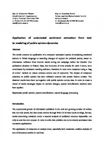
Because the Chao Phraya river basin is located in a large flat plain, inundation always remains for an extended period of time. The damage caused by flooding depends not only on the water depth but also on the flood duration. In 2011, the inundation depths ranged between 0.6 m and 4.9 m, with an average of 2.2 m, and the mode (most frequent value) was 2.5 m. Fifty-seven (57) days was the average inundation duration, which ranged from 3 to 120 days and had a mode of 60 days [3]. The flooded areas could be captured remotely by a single satellite image, and the duration could be obtained by monitoring the flooded areas in a sequence of time. However, water depth requires auxiliary data for processing, e.g., a digital elevation model (DEM). In this study, estimating water depth was set aside for future work. Thus, only the inundation area and duration are studied in this article. Working with multi-temporal SAR images, it is very difficult to obtain images in the exact same conditions, e.g., satellite position, look-side (right/left), and incidence angle. Several methods must be introduced to normalize multi-temporal images prior to analysis [32,33]. In contrast, the proposed method, which obtains the threshold value from water references, is independent of the acquisition condition, and there is no need to normalize the images [19–21]. 2. Study Area and Imagery Data This paper focuses on the Chao Phraya river basin in the central part of Thailand, which has an area of approximately 7400 km2 . The basin was assigned as a regularly inundated area by the Thai government. The city of Ayutthaya, which is approximately 16.5 km in width and 21.0 km in length and includes the Ayutthaya Historical Park and the Rojana and Hi-Tech Industrial Parks, was selected Remote Sens. 2017, 9, x FOR REVIEWwater bodies during the 2011 Thailand flood, as shown in Figure 4 of 19 as a validation area forPEER extracting 1.
River DEM 1127m
-1m
Figure 1. Map showing Figure 1. Map showing the the study study area area (left), (left), where where the the black black border border delimits delimits the the Chao Chao Phraya Phraya river river basin in central Thailand, and the red square delimits Ayutthaya City. Topographic map (middle), basin in central Thailand, and the red square delimits Ayutthaya City. Topographic map (middle), with with main main streams streams on on the the DEM. DEM. Water Water reference reference map map showing showing 87 87 water water references references throughout throughout the the study area on a RADARSAT-2 image (right). study area on a RADARSAT-2 image (right).
Tabledata 1. Summary of by theRADARSAT-2 RADARSAT-2 image properties used in thisseveral study. beam types, The imagery acquired (RS2)data during that event have i.e., Wide1 (W1), Wide2 (W2), Wide3 (W3), SCNA (W1 + W2), and SCNB (W2 + S5 + S6). The radar Incident Angle Number of frequency, resolution, and incident angle Swath variedWide depending on the beam(degrees) type. Most of the images Resolution Pixels/Lines Scenes were Beam / Swatch Position taken in the HH and HV dual-polarization mode, (m) (km) and 30 images using that polarization were selected. Near Far Asc. Des. The images were observed either from the ascending (ASC) or descending (DES) path. A summary of W1 (Wide1)
12.5
170
12,930
20.0
31.9
-
5
W2 (Wide2)
12.5
150
12,930
30.6
39.5
-
1
W3 (Wide3)
12.5
130
12,930
38.7
45.3
2
-
SCNA (ScanSAR W1 + W2)
25.0
300
12,000
20.0
39.5
7
6
300
12,000
Remote Sens. 2017, 9, 78
4 of 19
the image properties is presented in Table 1, and their color composite maps are shown in Figure 2. Because the swath width and revisit time of the satellite are limited, only some of the images could capture the whole area. Remote Sens. 2017, 9, xstudy FOR PEER REVIEW 5 of 19
1
2
7
3
4
5
6
9
10
11
12
13
14
15
16
17
18
19
20
21
22
23
24
25
26
27
29
30
28
Figure 2. RADARSAT-2 color composite (HH as red, HV as green, and HH/HV as blue) images taken Figure 2. 2011 RADARSAT-2 composite as red, HV as green, and HH/HV as blue) images taken during the Thai floodcolor event from the(HH beginning to end. during the 2011 Thai flood event from the beginning to end.
Remote Sens. 2017, 9, 78
5 of 19
Table 1. Summary of the RADARSAT-2 image data properties used in this study. Beam/Swatch Position
Resolution (m)
Swath Wide (km)
Pixels/Lines
12.5 12.5 12.5 25.0 25.0
170 150 130 300 300
12,930 12,930 12,930 12,000 12,000
W1 (Wide1) W2 (Wide2) W3 (Wide3) SCNA (ScanSAR W1 + W2) SCNB (ScanSAR W2 + S5 + S6)
Total
Incident Angle (degrees)
Number of Scenes
Near
Far
Asc.
Des.
20.0 30.6 38.7 20.0 30.6
31.9 39.5 45.3 39.5 46.5
2 7 4
5 1 6 5
13
17 30
Two optical images were also used for validation. A GeoEye-1 (GE1) image was prioritized because it had a higher resolution and was taken on 22 November 2011, which was the nearest in time to one of the RS2 images. The pan-sharpened GE1 image had four multispectral bands with a 1.0-m resolution. ThaiChote-1 (TH1) images are also important because they are used as common data. A pan-sharped TH1 image has a multispectral band with a 2.5-m resolution. A TH1 image was taken on 25 November 2011. Another TH1 image was taken prior the flood on 12 December 2009. That image was used to assess the environment in the dry season but was not used in the analysis process. All the optical images will be shown in the accuracy assessment section. 3. Methodology and Results The methodology used in this study is comprised of two parts. The main part is an automated system that extracts water bodies and produces flood duration maps. The second part is an accuracy assessment, which is a process to measure the efficiency of the main part using optical images as truth data. That part did not need to be implemented in the automated system. The main part begins with preparing RS2 images by the radiometric calibration using the lookup tables provided in these products, the Refined Lee speckle filtering [34,35] with a window size of 5 × 5 pixels, and the terrain correction using an SRTM 90-m DEM. Radiometric calibration provides images in which pixels can be directly related to the radar backscatter of the scene by applying the sigma naught, beta naught, and gamma naught lookup tables provided in the product [32]. The pre-processing was performed using the Sentinel Application Platform (SNAP) software program. Next, RS2 images were clipped by the study area and then temporarily cut again into specific segments throughout the study area. Those particular segments were defined as water references, as mentioned in the next section. The automatic thresholding was applied to each water reference one at a time to estimate a local threshold value. In that step, water references with unimodal distribution histograms were rejected. The local threshold values were weight-averaged by area to estimate the global threshold value. Finally, the global threshold value was applied to the whole image to extract the water bodies. The flood duration map is an auxiliary product for flood management and is calculated from the cumulative days of water bodies. All these processes were developed using a Python script and applicable modules, e.g., the Geospatial Data Abstraction Library (GDAL) for reading and writing image data, NumPy for numerical calculation, and Matplotlib for plotting histograms. NumPy is the fundamental package for scientific computing with powerful N-dimensional array objects and linear algebra. Matplotlib is 2D and 3D plotting library which produces quality figures under interactive environments. The purpose of the accuracy assessment was to measure the efficiency and accuracy of the final results by comparing the water areas extracted from the SAR images (RS2) with those from the optical images (GE1 and TH1). The backscattering coefficient was used for the SAR images, and the Normalized Difference Water Index (NDWI) was used for the optical images. Although the RS2 images were processed using automatic thresholding, the GE1 image was processed using manual thresholding. The RS2 and TH1 results were compared with the GE1 image to determine the most accurate thresholding. The work flow diagram used in this study is shown in Figure 3.
results by comparing the water areas extracted from the SAR images (RS2) with those from the optical images (GE1 and TH1). The backscattering coefficient was used for the SAR images, and the Normalized Difference Water Index (NDWI) was used for the optical images. Although the RS2 images were processed using automatic thresholding, the GE1 image was processed using manual thresholding. Remote Sens. 2017,The 9, 78RS2 and TH1 results were compared with the GE1 image to determine the most 6 of 19 accurate thresholding. The work flow diagram used in this study is shown in Figure 3. RADARSAT-2 RADARSAT2 RADARSAT2 HH, HV Water References Water References References
GEOEYE-1 / THAICHOTE-1 Calibration/ Speckle Filter
Bimodal Histogram Selection
NDWI Terrain correction Manual Thresholding
Automatic Thresholding Global Thresholding
Water Area
Threshold Values Water Areas RADARSAT2 RADARSAT2
Accuracy
Weight Average Threshold
Flood Duration Map
Figure 3. Work flow diagram for automatic flood extraction for RADARSAT-2. The optical image procedure shown by the dashed was used for extraction a one-time for accuracy assessment. Figure 3. Work flow diagram forlines automatic flood RADARSAT-2. The optical image procedure shown by the dashed lines was used for a one-time accuracy assessment.
3.1. Water References and Histogram Analysis 3.1. Water References and Histogram Analysis Applying automatic clustering-based thresholding to a large area may return unsatisfying results Applying automatic clustering-based thresholding to aproblem large area maywhen return because its histogram is not bimodally distributed [31]. This occurs theunsatisfying ratios of the results because its histogram is not bimodally distributed [31]. This problem occurs when the ratios water and non-water areas are very different. A novel technique was implemented in this study to of the water and non-water areas are very different. A novel technique was implemented in this overcome this problem by applying automatic thresholding to specific smaller areas located throughout study to overcome thissmall problem applying automatic to specific areas the study area. Those areasbywere defined as waterthresholding references, which can besmaller used for any located satellite throughout the study area. Those small areas were defined as water references, which can be used images acquired on a different date and time. for any satellite images acquired on a different date and time. All the water references were selected using the following criteria: having an area larger than 2 (512 All m the water references were selected the2048 following criteria: havingofan area than 320,000 pixels for a resolution of 25.0using m, and pixels for a resolution 12.5 m),larger containing 2 (512 pixels for a resolution of 25.0 m, and 2048 pixels for a resolution of 12.5 m), 320,000 m water throughout the year, not facing a flood situation, located on flat ground as much as possible, containing throughout the year, not facing a flood located onshape flat ground as much as and havingwater a water and non-water cover ratio of nearlysituation, 1:1. An irregular is allowed. In this possible, and having a water and non-water cover ratio of nearly 1:1. An irregular shape is allowed. study, an elliptical shape was preferred because it was easy to maintain the ratio of the water and In this study, an ellipticalThe shape was preferred because it was easy to different maintain types the ratio of thebodies, water non-water proportions. 87 water references were selected from of water and non-water proportions. 87 water references were 1selected natural and man-made. TheirThe locations are shown in Figure (right). from different types of water bodies, natural and man-made. Their locations are shown in Figure (right). Because not all of the RS2 images covered the entire study 1area and included all the water Because not all of the RS2 images covered the entire study area andbyincluded allimage the water references, only those water references whose entire areas were covered each RS2 were references, thoseThe water references whose entire areas covered by each image were taken into only account. number of water references and were their covering areas forRS2 each image are taken into account. The number of water references and their covering areas for each image are shown in Table 2. It was impossible to show all of them in this article, and thus only 10, taken on 28 February 2011, are shown in Figure 4 (see supplementary materials for the full version). Smooth water surfaces are shown in black for the HH, HV, and HH + HV polarizations and in deep blue for the color composites of HH, HV, and HH/HV. "HH + HV" denotes the sum of the backscattering coefficients as the total backscattering, and "HH/HV" denotes the ratio of the backscattering coefficients as the relative backscattering. Both values were calculated on a linear scale but are presented on a logarithmic scale (dB). The histogram plots shown in Figure 4 were obtained from the RS2 images and were clipped by the selected water reference within the red elliptical boundary. The blue curve shows the HH+HV backscattering coefficient, the red curve shows the HH backscattering coefficient, and the green curve shows the HV backscattering coefficient. Theoretically, these histograms should display a
Remote Sens. 2017, 9, 78
7 of 19
bimodal distribution, but some of them were found to have unimodal distributions. Examples include water surfaces covered by floating or emerged plants or surface waves caused by strong winds. These situations cause a larger than normal amount of SAR energy to be reflected back to the sensor [11–13]. This effect can be observed in the sample images for water references 024, 028, 063, and 076. By considering the peaks, valleys, and curvatures of the smoothed histograms, the water references with unimodal distributions were rejected, and only those with bimodal distributions were taken into account. The bimodal occurrences for the HH and HH + HV polarizations are shown in Table 2. This number indicates the occurrence probability of the bimodal distribution for each image. In that sense, HH + HV is more likely to have a bimodal distribution and is more suitable for automatic classification. In other words, the HV polarization can improve the efficiency of water surface extraction. Thus, the extracted water areas presented in this article were derived from HH + HV. Table 2. List of RADARSAT-2 images and threshold values for water extraction.
p
1 2 3 4 5 6 7 8 9 10 11 12 13 14 15 16 17 18 19 20 21 22 23 24 25 26 27 28 29 30
Local Time
2011/09/02 AM 2011/09/09 AM 2011/09/16 AM 2011/09/23 AM 2011/09/26 AM 2011/09/27 PM 2011/10/03 AM 2011/10/04 PM 2011/10/10 AM 2011/10/11 PM 2011/10/17 AM 2011/10/20 AM 2011/10/21 PM 2011/10/25 PM 2011/10/27 AM 2011/10/28 PM 2011/11/04 PM 2011/11/10 AM 2011/11/11 PM 2011/11/12 PM 2011/11/14 PM 2011/11/18 PM 2011/11/20 AM 2011/11/21 PM 2011/11/27 AM 2011/11/28 PM 2011/12/04 AM 2011/12/21 AM 2011/12/28 AM 2012/02/14 AM
Interval (days)
Path
7.0 7.0 7.0 3.0 1.5 5.5 1.5 5.5 1.5 5.5 3.0 1.5 4.0 1.5 1.5 7.0 5.5 1.5 1.0 2.0 4.0 1.5 1.5 5.5 1.5 5.5 17.0 7.0 48.0
DES DES DES DES DES ASC DES ASC DES ASC DES DES ASC ASC DES ASC ASC DES ASC ASC ASC ASC DES ASC DES ASC DES DES DES DES
Beam
Water References Count
W1 W1 W1 W2 W1 W3 W1 W3 SCNA SCNA SCNB SCNA SCNB SCNA SCNA SCNB SCNA SCNB SCNA SCNA SCNB SCNA SCNA SCNB SCNA SCNA SCNB SCNA SCNB SCNB
36 62 33 41 34 53 61 38 83 87 84 36 70 25 74 87 87 84 75 61 69 24 74 86 83 87 84 83 84 68
Bimodal Occurrences
Weighted-Average Threshold (dB)
Area (Km2 )
HH
HH + HV
HH
HH + HV
101.02 180.29 116.00 118.50 98.25 145.92 179.86 115.81 240.50 248.09 229.70 101.02 183.31 73.79 209.61 248.09 248.09 229.70 200.62 191.21 181.22 72.65 209.61 244.22 240.50 248.09 229.70 240.50 229.70 199.03
17/36 45/62 32/33 40/41 16/34 53/53 49/61 37/38 74/83 77/87 76/84 21/36 65/70 13/25 54/74 78/87 80/87 77/84 56/75 52/61 64/69 13/24 46/74 78/86 68/83 75/87 75/84 68/83 71/84 56/68
31/36 60/62 32/33 40/41 31/34 53/53 60/61 37/38 78/83 83/87 79/84 31/36 69/70 22/25 70/74 82/87 80/87 80/84 68/75 57/61 66/69 21/24 62/74 80/86 76/83 81/87 81/84 74/83 77/84 61/68
−1.25 −1.20 −1.37 −13.96 −1.01 −0.84 −0.98 −1.06 −1.27 −1.03 −1.07 −0.30 −0.92 −1.04 −1.05 −0.93 −1.17 −0.90 −1.04 −15.65 −1.16 −1.39 −1.24 −1.01 −1.46 −1.24 −1.21 −1.51 −1.30 −16.51
2.02 2.19 1.74 −12.87 2.06 2.21 2.26 2.01 1.92 2.04 2.00 2.50 2.08 2.18 2.07 2.14 1.94 2.10 2.04 −14.51 1.88 1.89 2.07 2.08 1.76 1.92 1.91 1.68 1.82 −15.26
Remote Sens. 2017, 9, 78 Remote Sens. 2017, 9, x FOR PEER REVIEW ThaiChote-1 HH,HV,HH/HV
HH+HV
8 of 19 9 of 19 HH
HV
Histogram Water 009
Water 024
Water 028
Water 031
Water 036
Water 046
Water 062
Water 063
Water 064
Water 076
Figure 4. Automated threshold values using the neighborhood valley method of water references in Figure 4. Automated threshold values using the neighborhood valley method of water references in the the red elliptical areas (10 of 87) from the HH, HV and HH + HV sigma-naught values taken on the red elliptical areas (10 of 87) from the HH, HV and HH + HV sigma-naught values taken on the evening evening of 28 November 2011 PM (1 of 30 in Table 2). The dashed lines represent unimodal of 28 November 2011 PM (1 of 30 in Table 2). The dashed lines represent unimodal distributions, distributions, and the solid lines represent bimodal distributions. The ThaiChote-1 images in the first and the solid lines represent bimodal distributions. The ThaiChote-1 images in the first column were column were acquired on different dates in the dry season. acquired on different dates in the dry season.
Remote Sens. 2017, 9, 78
9 of 19
3.2. Automatic Thresholding Otsu’s method (OT) is one of the best threshold selection methods for general gray-level images. 2 ) or the This technique chooses the threshold value of the minimum within-class variance (σW maximum between-class variance (σB2 ) in Equation (1). Although this method can obtain satisfactory segmentation results in many cases, it is basically limited to images with background and foreground Gaussian distributions of equal variance. Therefore, images that do not meet this criterion may return unsatisfactory results, especially when the gray level histogram is unimodal or close to a unimodal distribution [33]. To address this weakness, many modifications of the Otsu method have been proposed. For example, the valley-emphasis method (VE), modified by weight σB2 with p(t), the complement of a probability at a threshold value t, causes the valley in the histogram to be more likely to be better determined. The neighborhood valley-emphasis (NE) is an improvement of the valley-emphasis method by weighting σB2 with the neighborhood information in n = 2m + 1 intervals at the threshold value t as in Equation (2). The result is closer to the valley of the histogram because it considers the neighborhood around the threshold point in addition to the threshold point. The optimal threshold is chosen by maximizing the between-class variance function [17] as in Equation (3). σB2 (t) = pw (t)(µw (t) − µ)2 + pn (t)(µn (t) − µ)2 = pw pn (µw (t) − µn (t))2 ,
(1)
p(t) = p(t − m) + · · · p(t − 1) + p(t) + p(t + 1) + · · · p(t + m), and
(2)
t∗ = Arg max (1 − p(t)) σB2 (t)
(3)
where σB2 (t) is the between-class variance at threshold value t, µ is the mean value of all the intervals, µw (t) is the mean value of the water portion at threshold value t, µn (t) is the mean value of the non-water portion at threshold value t, pw (t) is the probability of the water portion at threshold value t, pn (t) is the probability of the non-water portion at threshold value t, m is the number of neighborhood intervals for threshold value t, p(t) is the probability of the interval at threshold value t, p(t) is the sum of the probabilities of the neighborhood interval around threshold value t, Arg max is the argument of the maxima for threshold value t in the function, and t∗ is the optimum threshold value. From the previous study [17] and our empirical test for all the images using three thresholding methods (OT, VE, and NE), the NE method yielded the most suitable result for water extraction from the RS2 images. The threshold value of that method was close to the valley of the histogram and was able to extract water surfaces quite well. Consequently, the NE method was used for automatic thresholding in the following discussion. All the histograms were calculated by dividing the entire range of values into 256 intervals and then setting the number of neighborhood intervals to 11 (m = 5). The results of the threshold values are displayed as vertical lines in the histogram plots in Figure 4. In the figure, the solid lines represent bimodal distributions, whereas the dashed lines represent unimodal distributions, which were excluded from the calculation of the global threshold. For example, water reference 076 was rejected when calculating the global threshold for HH + HV. The threshold values obtained from the bimodal distributions are the area-weighted average, resulting in the global threshold value. This threshold is expected to be effective for the entire image. All the global threshold values are listed in columns 10 and 11 of Table 2.
Remote Sens. 2017, 9, 78
10 of 19
Among the 30 RS2 images, the global threshold values were slightly different. This may be because the RS2 images were acquired under different conditions. Different paths result in different azimuth angles, whereas different beam modes result in different incident angles, wave frequencies, and image resolutions. Those conditions produce different backscattering coefficients. The proposed technique has less bias for selecting the threshold value because it does not depend on the satellite mode and seasonal environment. Thus, the extracted water bodies for all the acquisition dates can be combined. 3.3. Water Area Extraction and Flood Duration Map The water areas were simply extracted by applying a global threshold value to each RS2 image. Close-ups of the extracted result from the image acquired on 28 November 2011 are shown in Figure 5. The water boundaries obtained using this technique appear to be reasonable in comparison to the visually classified results from the original RS2 and TH1 images acquired in a dry season. All the RS2 images from the 30 dates were processed separately. Because some RS2 images did not cover the entire study area, the missing parts were estimated from the previous image. The results are shown in Figure 6. The results from the current date are shown in deep blue, and the estimated results from the previous date are shown in light blue. The estimations coincided with the actual flood situation; flooding began in the north region on 2 October 2011 (image 1), the flooded areas spread to the south on 23 October 2011 (image 4), the flood in the north had abated by 21 November 2011 (image 28), and was completely finished on 14 February 2012 (image 30). Remote Sens. 2017, 9, x FOR PEER REVIEW 11 of 19
Water 009
Water 024
Water 028
Water 031
Water 036
Water 046
Water 062
Water 063
Water 064
Water 076
Figure 5.5. Close-ups extents from the the RADARSAT-2 image acquired on Figure Close-upsofofthe theextracted extractedwater water extents from RADARSAT-2 image acquired 28 November 2011 using the HH+HV global threshold value (1.92 dB). The water areas are displayed on 28 November 2011 using the HH + HV global threshold value (1.92 dB). The water areas are in deep blue, and the red ellipses are the water references. displayed in deep blue, and the red ellipses are the water references.
4. Accuracy Assessment Flooding usually occurs over a long duration because the central region of Thailand is nearly flat. The accuracy of a classification be assessed by comparing the results with truth In Agricultural plants have limited times must to tolerate waterlogging or submerging. Buildings and data. electrical this study, are optical images that captured ground surface gagingThe stations that of recorded equipment not designed to work in this situation andactivity are hardand to repair. severity damage water heights were introduced as truth data sources. During this flood event, almost all the country to assets increases with flood duration. Therefore, the period of inundation or a flood duration map covered by clouds, satellitefor clear-sky images therefore were very rare. GeoEye-1 iswas very important to the and Thaioptical government controlling floods and developing remedial plans. (GE1) and ThaiChote-1 (TH1) clear-sky images taken on 22 November 2011 over Ayutthaya city The flood duration map was produced by stacking the interval of the extracted water surfaces. were selected the truth data. Those data covered Ayutthaya Historical theduration Rojana The final floodas duration map is shown in Figure 7. the Flooding usually occurs Park over and a long and Hi-Tech industrial parks, which are very important economically and for tourism. because the central region of Thailand is nearly flat. Agricultural plants have limited times to tolerate To extract the flooded areas from the optical images, using the Normalize Different Water Index waterlogging or submerging. Buildings and electrical equipment are not designed to work in this (NDWI) calculated from the Green (G) and near-infrared (NIR) band values is the most popular and situation and are hard to repair. The severity of damage to assets increases with flood duration. effective method [36]. McFeeters proposed the NDWI in 1996 to detect surface waters in wetland environments and to allow for the measurement of surface water extent, and asserted that values of NDWI greater than zero are assumed to represent water surfaces, while values less than, or equal to, zero are assumed to be non-water surfaces [37]. In this image interpretation, rivers and ponds were also extracted as flooded areas because nearly the entire study area was covered by water. The GE1 NDWI threshold for the water areas during the flood period was determined by visual
Remote Sens. 2017, 9, 78
11 of 19
Therefore, the period of inundation or a flood duration map is very important to the Thai government Remote Sens. 2017, 9, x FOR PEER REVIEW 12 of 19 for controlling floods and developing remedial plans. The flood duration map was produced by stacking the interval of the extracted water surfaces. The final flood duration map is shown in Figure 7.
1
2
3
4
5
6
7
8
9
10
11
12
13
14
15
16
17
18
19
20
21
22
23
24
25
26
27
28
29
30
Figure 6. Extracted water areas after applying the global threshold value for each Radarsat-2 image. Figure 6. Extracted water after applying the global threshold value for each Radarsat-2 image. The extracted results fromareas the actual date are shown in deep blue, and the results from the previous The extracted results from the actual date are shown in deep blue, and the results from the previous date are shown in light blue. date are shown in light blue.
Remote Sens. 2017, 9, 78 Remote Sens. 2017, 9, 78 Remote Sens. 2017, 9, x FOR PEER REVIEW
Duration (Days) 176
Duration (Days) 176
C35
C37
1
12 of 19
1
C37
C35 S5
12 of 19 13 of 19
S5
RID Gaging Station Ayutthaya Park Rojana Park Industrial Estate Industrial Hi-Tech Industrial Estate Industrial Estate RID Gaging StationHistorical Ayutthaya Historical Rojana Estate Hi-Tech
Figure 7. 7. Water Water duration duration map map calculated calculated by stacking The red red border border Figure 7. Water duration map calculated by stacking the extracted water surfaces. The red border Figure by stacking the the extracted extracted water water surfaces. surfaces. The shows Ayutthaya City, an enlargement of which is shown on the right side of the figure. The yellow shows Ayutthaya City, an enlargement of which is shown on the right side of the figure. The yellow shows Ayutthaya City, an enlargement of which is shown on the right side of the figure. The yellow border shows shows the the Rojana Rojana industrial industrial park. border shows the Rojana industrial park. border park.
4. Accuracy Assessment 4. Accuracy Similar Assessment to GE1, TH1 has an optical sensor with four bands with quite similar spectral ranges, but its spatial resolution is much lower. calculating the NDWI TH1truth image in Figure The accuracy of a classification must be assessed by comparing the results with truth data. In The accuracy of a classification mustBefore be assessed by comparing thevalues, results awith data. In this 8 (5A) was up-sampled and co-registered to the GE1 image. We then compared the NDWI in Figure this study, optical images that captured ground surface activity and gaging stations that recorded study, optical images that captured ground surface activity and gaging stations that recorded water 8heights (5B) with that from the GE1 image. The most accurate TH1 NDWI threshold for water was found water heights were introduced as truth data sources. During this flood event, almost all the country were introduced as truth data sources. During this flood event, almost all the country was to be 0.28, corresponds to 64.6% clear-sky of the estimated waterwere areas (W-W and N-W) in Figure 9(2A– was covered by clouds, and optical satellite clear‐sky images therefore very rare. GeoEye‐1 covered bywhich clouds, and optical satellite images therefore were very rare. GeoEye-1 (GE1) and 2C). Among those extracted areas, 85.2% were similar to those from the GE1 (W-W and N-N), 9.6% (GE1) and ThaiChote‐1 (TH1) clear‐sky Ayutthaya city city were selected ThaiChote-1 (TH1) clear-skyimages imagestaken takenon on22 22November November 2011 2011 over over Ayutthaya were negatives (W-N), and 5.1% were false positives (N-W). Park By applying NDWI were selected as the truth data. Those data covered the Ayutthaya Historical Park and the Rojana as thefalse truth data. Those data covered the Ayutthaya Historical and thethis Rojana andthreshold Hi-Tech to the TH1 pre-flood image, the water-covered ratio of this area was 11.9%. and Hi‐Tech industrial parks, which are very important economically and for tourism. industrial parks, which are very important economically and for tourism. For thresholding SARareas sensors, (the sigmaDifferent naught value, σ°) is To extract the flooded areas from the optical images, using the Normalize Different Water Index To extract the flooded fromthe thebackscattering optical images,coefficient using the Normalize Water Index used more often than the the NDWI for(G) optical The best threshold for theisRS2 HH+HV acquired (NDWI) calculated from the Green (G) and near‐infrared (NIR) band values is the most popular and (NDWI) calculated from Green and sensors. near-infrared (NIR) band values the most popular and on November 21, 2011 was determined to be 3.18 dB, which corresponds to 64.9% of the estimated effective method [36]. McFeeters proposed the proposed NDWI in the 1996 to detect surface waters in wetland effective method [36]. McFeeters NDWI in 1996 to detect surface waters in wetland water areas (W-W N-W). those extracted waterwater areas,extent, 79.9% and wereasserted similar that to the results environments and to allow for the measurement of surface water extent, and asserted that values of environments and and to allow forAmong the measurement of surface values of from GE1 (W-W and N-N), 12.2% were false negatives (W-N), and 7.9% were false positives (N-W). NDWI greater than zero are assumed to represent water surfaces, while values less than, or equal to, NDWI greater than zero are assumed to represent water surfaces, while values less than, or equal to, zero are assumed to be non‐water surfaces [37]. In this image interpretation, rivers and ponds were zero are assumed to be non-water surfaces [37]. In this image interpretation, rivers and ponds were 4.2. Comparison between the Best Accuracy Method and the Proposed Method also extracted as flooded areas because nearly the entire study area was covered by water. The GE1 also extracted as flooded areas because nearly the entire study area was covered by water. The GE1 NDWI threshold for the water areas during the flood period was determined visual NDWI threshold forvalue the water areas during the accurate flood period was determined by visual interpretation The threshold for RS2 from the most thresholding methodby was greater, covered a interpretation of Figure 8(4B) as NDWI ≧ 0.02 or 69.1% of the image area shown in Figure 9(1A–1C). of Figure 8(4B) as NDWI 0.02 accurate or 69.1% of the image area shown in Figure 9(1A–1C). This NDWI larger area and was more than the proposed weight averaged neighborhood This NDWI threshold value was used as the truth data when obtaining the most accurate threshold threshold value was used as the truth data obtainingvalue the most accurate values for valley-emphasis thresholding method. The when RS2 threshold acquired for threshold 21 November 2011, values for NDWI from TH1 and HH + HV from RS2. NDWI from TH1the and HHaccurate + HV from RS2. (image 24) from most thresholding method was 3.18 dB (64.9% area coverage), whereas
that by the proposed method was 2.08 dB (44.0% area coverage). For the proposed method, 71.9% of the results were similar to the results of GE1 (W-W and N-N), 26.6% were false negatives (W-N), and 1.5% were false positives (N-W). From Figure 9(3B,3C), the blue color shows the water areas extracted by the proposed method, and the green color shows the difference from the best accuracy method. Although the threshold value of the best accuracy method is apparently more eligible, applying that local threshold value to the entire study area returned an inappropriate result and was difficult to implement as a practical procedure. The extraction of water surfaces using that threshold value for the entire area resulted in overestimation. For example, the water areas in Figures 5 and 6 became noisier. Moreover, it was almost impossible to find suitable optical images to be used as references for the SAR images throughout the event.
Remote Sens. Remote Sens.2017, 2017,9,9,78 x FOR PEER REVIEW Remote Sens. 2017, 9, x FOR PEER REVIEW
13 19 of 19 14 of 14 of 19 GEOEYE-1 GEOEYE-1
1B 1B
1A 1A
AM 2011/11/22 AM 2011/11/22
PM 2011/11/21 PM 2011/11/21
RADARSAT-2 RADARSAT-2
4A 4A
4B 4B
3A 3A
3B 3B
HH HH
HV HV
HH/HV HH/HV
HH+HV 4 HH+HV 4
40dB 40dB
AM 2011/11/25 AM 2011/11/25
2B 2B
5A 5A
5B 5B
AM 2009/12/13 AM 2009/12/13
AM 2011/11/27 AM 2011/11/27
2A 2A
AM 2012/02/14 AM 2012/02/14
THAICHOTE THAICHOTE
6A 6A
6B 6B NDWI −1 NDWI −1
False color False color
1 1
Figure8.8.Close-up Close-up of Ayutthaya city city for in-flood in-flood and post-flood time. The color Figure Thedual dualpolarization polarization color Figure 8. Close-upofofAyutthaya Ayutthaya cityfor for in-flood and and post-flood post-flood time. time. The dual polarization color composite (1A–3A) and HH + HV (1B–3B) from RADARSAT-2. The false color composite and composite (1A–3A) and HHHH + HV (1B–3B) fromfrom RADARSAT-2. The false color color composite and NDWI composite (1A–3A) and + HV (1B–3B) RADARSAT-2. The false composite and NDWI (4A, 4B) from GeoEye-1, and the false color composite and NDWI for in-flood (5A, 5B) and (4A, 4B) from and the false composite and NDWI in-flood 5B) (5A, and pre-flood NDWI (4A, GeoEye-1, 4B) from GeoEye-1, and color the false color composite andfor NDWI for (5A, in-flood 5B) and pre-flood (6A, 6B) times from ThaiChote-1. (6A, 6B) times from pre-flood (6A, 6B) ThaiChote-1. times from ThaiChote-1. FREQUENCY FREQUENCY Pixels Pixels
CUMULATIVE CUMULATIVE
FREQUENCY FREQUENCY Pixels Pixels
69.1 % 69.1 % In-flood In-flood NDWI NDWI
GEOEYE-1 (2011/11/22 AM) GEOEYE-1 (2011/11/22 AM)
1A 1A Pix Pix
NDWI NDWI
CUMULATIVE CUMULATIVE Pre-flood Pre-flood 11.9 % 11.9 % In-flood In-flood 64.6% 2A 64.6% 2A Pix Pix
FREQUENCY FREQUENCY Pixels Pixels
HH+HV HH+HV
CUMULATIVE CUMULATIVE In-flood In-flood 44.0% 44.0% Post-flood Post-flood 27.6% 27.6%3A 3A Pix Pix
1B 1B
2B 2B
3B 3B
1C 1C
2C 2C THAICHOTE-1 (2011/11/25 AM) THAICHOTE-1 (2011/11/25 AM)
3C 3C RADARSAT-2 (2011/11/21 PM) RADARSAT-2 (2011/11/21 PM)
Figure 9. Histograms and cumulative probability plots (top) and extracted flooded areas (blue color) in Figure 9. Histograms andand cumulative probability plots (top) and extracted flooded areas (blue color) in Figure 9. Histograms cumulative (top) and extracted (blue color) Ayutthaya city (middle) and over part of probability the Rojana plots Industrial Park (bottom),flooded from theareas visualization of in Ayutthaya citycity (middle) andand over partpart of the Rojana Industrial Park (bottom), from the the visualization of over of the Industrial Park (bottom), from visualization the Ayutthaya GeoEye-1 image(middle) (1A–1C), determining the bestRojana accuracy of the ThaiChote-1 image (2A–2C), and the theofGeoEye-1 imageimage (1A–1C), determining the best accuracy of theofThaiChote-1 imageimage (2A–2C), and the the GeoEye-1 (1A–1C), determining the best accuracy the ThaiChote-1 (2A–2C), and emphasis of the neighborhood valley on the RADARSAT-2 image (3A–3C), plotted on a GeoEye-1 false emphasis of the neighborhood valley on the on RADARSAT-2 image image (3A–3C), plottedplotted on a GeoEye-1 false the emphasis of the neighborhood the best RADARSAT-2 (3A–3C), a GeoEye-1 color composite. The green pixels are thevalley determined accuracy results from RADARSAT-2,onwhich was color composite. The green pixels are the determined best accuracy results from RADARSAT-2, which was false color green pixels are the determined best method. accuracy results from RADARSAT-2, larger than thatcomposite. determinedThe using the neighborhood valley-emphasis larger than that determined using the neighborhood valley-emphasis method. which was larger than that determined using the neighborhood valley-emphasis method.
Remote Sens. 2017, 9, 78
14 of 19
4.1. Finding the Best Accuracy Thresholds for the ThaiChote-1 and RADARSAT-2 Images The comparison of two (the truth data and estimation) two-class spatial images, water areas (W) or non-water areas (N) results in four combinations: W-W, N-N, W-N, and N-W. When the threshold for a client’s image is set to the minimum value, all of the results will be non-water areas (N). Some of them are N-N, which represents the same N values as those from the master image (GE1), whereas the others are W-N, which represents a water extraction omission error (false negative). When the threshold of the client image moves to higher values, some values will be considered to be water (W). Some of these values are W-W, which represent the same W values, whereas the others are N-W, which represent overestimation (commission error, false positive) in the water extraction. The best threshold value is the point where the summation of the W-W and N-N areas becomes largest. This point corresponds to the result most similar to that from the GE1 image. The results of this approach are shown in Table 3. Table 3. Results of the accuracy assessment of the water extraction for Ayutthaya city. Satellite/Date
Data
Method
Threshold Value
N-N (%)
W-N (%)
N-W (%)
W-W (%)
Water (N-W + W-W) (%)
Accuracy (N-N + W-W) (%)
GE1 2011/11/22 AM TH1 2011/11/25 AM RS2 2011/11/21 PM
NDWI NDWI HH+HV
VS (1) BA (2) BA (2) NE (3)
0.02 0.28 3.18 dB 2.08 dB
25.8 23.0 29.4
9.6 12.2 26.6
5.1 7.9 1.5
59.5 56.9 42.4
69.1 64.6 64.9 44.0
85.2 79.9 71.9
(1) VS = visualization thresholding; (2) BA = find best accuracy thresholding; (3) NE = weight-average neighborhood valley-emphasis thresholding.
Similar to GE1, TH1 has an optical sensor with four bands with quite similar spectral ranges, but its spatial resolution is much lower. Before calculating the NDWI values, a TH1 image in Figure 8(5A) was up-sampled and co-registered to the GE1 image. We then compared the NDWI in Figure 8(5B) with that from the GE1 image. The most accurate TH1 NDWI threshold for water was found to be 0.28, which corresponds to 64.6% of the estimated water areas (W-W and N-W) in Figure 9(2A–2C). Among those extracted areas, 85.2% were similar to those from the GE1 (W-W and N-N), 9.6% were false negatives (W-N), and 5.1% were false positives (N-W). By applying this NDWI threshold to the TH1 pre-flood image, the water-covered ratio of this area was 11.9%. ◦ For thresholding SAR sensors, the backscattering coefficient (the sigma naught value, σ ) is used more often than the NDWI for optical sensors. The best threshold for the RS2 HH+HV acquired on November 21, 2011 was determined to be 3.18 dB, which corresponds to 64.9% of the estimated water areas (W-W and N-W). Among those extracted water areas, 79.9% were similar to the results from GE1 (W-W and N-N), 12.2% were false negatives (W-N), and 7.9% were false positives (N-W). 4.2. Comparison between the Best Accuracy Method and the Proposed Method The threshold value for RS2 from the most accurate thresholding method was greater, covered a larger area and was more accurate than the proposed weight averaged neighborhood valley-emphasis thresholding method. The RS2 threshold value acquired for 21 November 2011, (image 24) from the most accurate thresholding method was 3.18 dB (64.9% area coverage), whereas that by the proposed method was 2.08 dB (44.0% area coverage). For the proposed method, 71.9% of the results were similar to the results of GE1 (W-W and N-N), 26.6% were false negatives (W-N), and 1.5% were false positives (N-W). From Figure 9(3B,3C), the blue color shows the water areas extracted by the proposed method, and the green color shows the difference from the best accuracy method. Although the threshold value of the best accuracy method is apparently more eligible, applying that local threshold value to the entire study area returned an inappropriate result and was difficult to implement as a practical procedure. The extraction of water surfaces using that threshold value for the entire area resulted in overestimation. For example, the water areas in Figures 5 and 6 became noisier.
Remote Sens. 2017, 9, 78
15 of 19
Moreover, it was almost impossible to find suitable optical images to be used as references for the SAR images throughout the event. Remote Sens. 2017, 9, x FOR PEER REVIEW
15 of 19
4.3. Comparison with the Gaging Station Data
Because the satellite images were not taken from the same sensors and were not acquired on the Table 3. Results of the accuracy assessment of the water extraction for Ayutthaya city. same date, it is difficult to explain the cause of the different extracted water extents. The difference in Water Accuracy sensor types and spatial resolutions and changes in water height over time may have contributed to the Threshold N-N W-N N-W W-W Satellite/Date The heights Data of Method (N-W flows + W-W) downward (N-N + W-W) discrepancy. the flood waters were difficult to project because water Value (%) (%) (%) (%) (%)the flood(%) without stopping, although water flows rather slowly in this area. To understand event, (1) GE1 2011/11/22 AM NDWI VS 0.02 69.1 the daily average water heights above the mean sea level (MSL) that were collected from the- three TH1 2011/11/25 AM NDWI stations BA (2) (C35, C37, 0.28 and S5) 25.8and recorded 9.6 5.1 59.5 Irrigation 64.6 85.2 nearest telemetry gaging by the Royal Department (2) RS2 2011/11/21 PM theHH+HV BA from the 3.18 dB 12.2 at four 7.9 checkpoints 56.9 64.9 (RID) [38] and water depths surface23.0 of the road reported by 79.9 Rojana Industrial Park Public Co., Ltd. introduced NE (3)[39] were 2.08 dB 29.4 as truth 26.6 data, 1.5 as shown 42.4 in Figure 44.0 10. The 71.9four water werethresholding; located in the Industrial Park at the power(3)plant Rojana phase-1 (1) checkpoints VS = visualization (2) Rojana BA = find best accuracy thresholding; NE (RJ0), = weight-average gate-A in front valley-emphasis of the head office (RJ1), Rojana phase-2 gate-B (RJ2), and Rojana-3 around the flyover neighborhood thresholding. (RJ3). Among them, RJ0 was closest to the Honda automobile factory shown in Figure 9. MSL (m)
MSL (m)
Station Levee (MSL) S5 C35 C37
4.70 4.58 3.80
Water Height (MSL)
Water Depth Above Levee (Meter)
Water Depth Above Road (Meter)
Satellite Images
Acquired Date
S5
C35
C37
S5
C35
C37
RJ0
RJ1
RJ2
RJ3
RADARSAT-2 GeoEye-1 ThaiChote-1
2011/11/21 2011/11/22 2011/11/25
4.56 4.48 4.17
4.65 4.56 4.25
4.7 4.62 4.41
-0.14 -0.22 -0.53
0.07 -0.02 -0.33
0.90 0.82 0.61
0.80 0.69 0.00
0.69 0.58 0.00
0.82 0.68 0.29
1.02 0.90 0.46
Figure Figure10. 10.Comparison Comparisonofofthe thewater waterheights heightsrecorded recordedatatthree threetelemetry telemetrygaging gagingstations stationsand andthe thelevee levee heights heights(left); (left);enlargement enlargementofofthe theleft leftplot plotfor for14–27 14–27October Octoberand andthe thewater waterdepths depthsabove abovethe theroad road surface surfaceobserved observedatatfour fourcheckpoints checkpointsininthe theRojana RojanaIndustrial IndustrialPark Park(right). (right).
4.3. Comparison The solidwith linesthe inGaging the leftStation graphData show the water heights at the three telemetry gaging stations
over a one-year period (April March 2012). period over which the satellite images Because the satellite images2011 weretonot taken fromThe the same sensors and were not acquired on were the acquired the endto ofexplain the flood event, thedifferent water level had dramatically decreased. Although same date,was it isatdifficult the causewhen of the extracted water extents. The difference water heights slightly different 22 November they hadtime significantly more inthe sensor types andwere spatial resolutions andon changes in water2011, height over may havedropped contributed than 30 cm in three days by 25 November 2011. to the discrepancy. The heights of the flood waters were difficult to project because water flows Because Ayutthaya is situated on awater relatively flatrather plain,slowly a smallinincrease in the height the may downward without stopping, although flows this area. To water understand cause the water to spread over a wide area. At that time, only the water at station C37 was higher than flood event, the daily average water heights above the mean sea level (MSL) that were collected from thethree levee, and the water atgaging this station spread theS5) river. thethe water heights at the the nearest telemetry stations (C35,beyond C37, and and Although recorded by Royal Irrigation other stations (S5 and C35) were below the height of the levee and no water spread outside, the water Department (RID) [38] and the water depths from the surface of the road at four checkpoints remained on the ground. At water checkpoint RJ0, in front of the power plant and close to the Honda reported by Rojana Industrial Park Public Co., Ltd. [39] were introduced as truth data, as shown in automobile factory, the water depth above road in surface was 0.80 m on November 21 power and deceased Figure 10. The four water checkpoints werethe located the Rojana Industrial Park at the plant to 0.69 m on 22 November and the water had completely drained by November 25. The extracted areas (RJ0), Rojana phase-1 gate-A in front of the head office (RJ1), Rojana phase-2 gate-B (RJ2), and determined in this study may have been slightly different because the satellite images were acquired Rojana-3 around the flyover (RJ3). Among them, RJ0 was closest to the Honda automobile factory on different dates. shown in Figure 9. The solid lines in the left graph show the water heights at the three telemetry gaging stations over a one-year period (April 2011 to March 2012). The period over which the satellite images were acquired was at the end of the flood event, when the water level had dramatically decreased. Although the water heights were slightly different on 22 November 2011, they had significantly dropped more than 30 cm in three days by 25 November 2011.
Remote Sens. 2017, 9, 78
16 of 19
5. Discussion and Future Work The proposed method can improve the speed of automated thresholding because to determine the global threshold value from static local areas is much more efficient than to do from systematic hierarchical local areas. This technique is suitable for multi-temporal images in a specific place, like the Chao Phraya river basin. Although the processing for permanent water references is rapid, the selection of proper water references takes time at the first step. An improper water reference without a bimodal distribution histogram should not be considered because it does not contribute to the estimation of the global thresholding. Open water from SAR images can be extracted quite well, but it is difficult to extract water in inundated urban areas and under trees [25,27,40]. The most important factor that limits the use of satellite data are resolution. When a satellite records data in a high-resolution mode, the imaging swath becomes smaller than that in the normal mode. This fact is caused by limitations of the data recorder and transmitter. Observing an inundation over a wide area with the same sensor or the same satellite is almost impossible. Although RS2 can observe in the spotlight mode at a 1-m resolution, the image on November 22 was acquired in the SCNB mode at a 25-m resolution to cover a larger area. On the other hand, the resolutions of pan-sharpened GE1 and TH1 images are 1 m and 2 m, respectively. Therefore, the GE1 and RS2 results are quite different (approximately 23–33%), according to the accuracy assessment. For detecting the water surface, a large number of pixels were missing because the overall backscattering of the pixels surrounded by obstacles such as buildings was higher than for open spaces. Sensor type can also cause differences. Although the NDWI obtained from optical sensors is suitable for the detection of water surfaces, objects having low infrared radiation are also classified as water surfaces. This misclassification can be observed in Figure 9(1C) and (2C). The roof-tops of buildings were sometimes identified as flood water by GE1, and there were more false-positive classifications from TH1. Water surfaces may also be misclassified by the backscattering coefficient from a SAR sensor. For example, non-water objects with smooth surfaces such as roads and runways are classified as water surfaces. Furthermore, side-looking transmission hinders observational ability. Water surfaces next to buildings produce double bounce backscattering, resulting in a total backscattering coefficient that is higher than usual and misclassifications as non-water. This effect can be observed in Figure 9(3C), where the west sides of the buildings were misclassified because the layover was projected onto the water surface. Similarly, the water surfaces between the buildings were misclassified. Observing inundations using satellites has another drawback; water under roofs or inside buildings cannot be observed. Auxiliary data must be prepared to provide the missing information. The average ground elevation data were prepared from an aerial survey conducted by the Japan International Cooperation Agency (JICA) for the zone along the Chao Phraya river and by ESRI Thailand for the outer area in 2012. The combined data can cover the entire Chao Phraya river basin. Future research needs to focus on improving accuracy through the utilization of LiDAR DEMs as topographic data. 6. Conclusions Multi-temporal RADARSAT-2 images with different acquisition conditions were used to extract water areas from the 2011 central Thailand flood along the Chao Phraya river. Considering the use of satellite SAR data in emergency situations, where validation data are scarce and optical images are hindered by cloud cover, an automated thresholding approach for water extraction was attempted. By introducing the global threshold value of the entire study area for each SAR image, the weight-averaged neighborhood valley-emphasis method was able to extract flooded areas automatically from the backscattering coefficient. The proposed method, which obtains the threshold value from the water references located throughout the Chao Phraya river basin, is more suitable for Thailand. Moreover, this technique is independent of the satellite acquisition condition,
Remote Sens. 2017, 9, 78
17 of 19
and there is no need to normalize the images before combining all the extracted water-areas as a flood duration map. In this case, the HH+HV dual-polarization achieved a higher accuracy than the HH single-polarization for open water extraction, which is affected by winds and floating/submerged plants. The extraction result for Ayutthaya city was similar to the visual inspection result from a GeoEye-1 image (approximately 67%), whereas the result obtained by the best accuracy thresholding method was approximately 77%. The results based on the ThaiChote-1 image were more similar to that from the GeoEye-1 image (approximately 82%) because they were both obtained by high-resolution optical satellites. On the other hand, the results from RADARSAT-2 had lower accuracies than those from GeoEye-1 and ThaiChote-1 because of its lower spatial-resolution and side-looking observational scheme. SAR images also have limitations for observing water areas covered by trees or adjacent to buildings. Despite these obstacles, the extraction of flooded areas from SAR intensity data can be improved by introducing pre-event topographic data such as LiDAR DEMs and building footprints. Supplementary Materials: The following are available online at http://www.mdpi.com/2072-4292/9/1/78/s1. For Figure 4: Automated threshold values determined using the neighborhood valley method for all the water references and for all the RADARSAT-2 images. Acknowledgments: This study was financially supported by the Grants-in-Aid for Scientific Research (project numbers 24241059). All the imagery data were provided by Geo-Informatics and Space Technology Development Agency (GISTDA), Thailand. Author Contributions: Pisut Nakmuenwai and Fumio Yamazaki conceived and designed the experiments; Pisut Nakmuenwai performed the experiments and analyzed the data; Fumio Yamazaki and Wen Liu contributed reagents/materials/analysis tools; Pisut Nakmuenwai wrote the paper.
References 1.
2.
3.
4.
5.
6.
7. 8. 9. 10. 11.
AON Benfield. 2011 Thailand Floods Event Recap Report, Impact Forecasting; Impact Forecasting LLC: Chicago, IL, USA, 2012; p. 40. Available online: http://thoughtleadership.aonbenfield.com/Documents/20120314_ impact_forecasting_thailand_flood_event_recap.pdf (accessed on 31 October 2016). The World Bank. Thai Flood 2011 Rapid Assessment for Resilient Recovery and Reconstruction Planning; The World Bank: Nonthaburi, Thailand, 2012; Volume 2, p. 377. Available online: http://documents. worldbank.org/curated/en/262141468118140200/pdf/698220WP0v20P10se0Only060Box370022B.pdf (accessed on 31 October 2016). Japan International Cooperation Agency (JICA). Project for the Comprehensive Flood Management Plan for the Chao Phraya River Basin, Final Report: Main Report; JICA: Tokyo, Japan, 2012; Volume 2, p. 219. Available online: http://open_jicareport.jica.go.jp/pdf/12127213_01.pdf (accessed on 31 October 2016). Henderson, F.M.; Lewis, A.J. Introduction. In Principles and Applications of Imaging Radar. Manual of Remote Sensing, 3rd ed.; Henderson, F.M., Lewis, A.J., Eds.; John Wiley & Sons, Inc.: New York, NY, USA, 1998; Volume 2, pp. 1–6. Rakwatin, P.; Sansena, T.; Marjang, N.; Rungsipanich, A. Using multi-temporal remote-sensing data to estimate 2011 flood area and volume over Chao Phraya River Basin, Thailand. Remote Sens. Lett. 2013, 4, 243–250. [CrossRef] Auynirundronkool, K.; Chen, N.; Peng, C.; Yang, C.; Gong, J.; Silapathong, C. Flood detection and mapping of the Thailand Central Plain using RADARSAT and MODIS under a sensor web environment. Int. J. Appl. Earth Obs. Geoinf. 2012, 14, 245–255. [CrossRef] Pierdicca, N.; Chini, M.; Pulvirenti, L.; Macina, F. Integrating physical and topographic information into a fuzzy scheme to map flooded area by SAR. Sensors 2008, 8, 4151–4164. [CrossRef] [PubMed] Pierdicca, N.; Pulvirenti, L.; Chini, M.; Guerriero, L.; Candela, L. Observing floods from space: Experience gained from COSMO-SkyMed observations. Acta Astronaut. 2013, 84, 122–133. [CrossRef] Brisco, B.; Short, N.; van der Sanden, J.; Landry, R.; Raymond, D. A semi-automated tool for surface water mapping with RADARSAT-1. Can. J. Remote Sens. 2009, 35, 336–344. [CrossRef] Bolanos, S.; Stiff, D.; Brisco, B.; Pietroniro, A. Operational surface water detection and monitoring using Radarsat 2. Remote Sens. 2016, 8, 285. [CrossRef] Lee, J.; Grunes, M.R.; Pottier, E. Quantitative comparison of classification capability: Fully polarimetric versus dual and single-polarization SAR. IEEE Trans. Geosci. Remote Sens. 2001, 39, 2343–2351.
Remote Sens. 2017, 9, 78
12.
13. 14. 15. 16. 17. 18. 19.
20. 21. 22.
23.
24. 25. 26.
27.
28.
29.
30.
31. 32.
18 of 19
Kim, S.-B.; Ouelette, J.D.; Zyl, J.; Johnson, J.T. Detection of inland open water surfaces using dual polarization L-band radar for the soil moisture active passive mission. IEEE Trans. Geosci. Remote Sens. 2016, 54, 3388–3399. [CrossRef] Martinis, S.; Rieke, C. Backscatter analysis using multi-temporal and multi-frequency SAR data in the context of flood mapping at River Saale, Germany. Remote Sens. 2015, 7, 7732–7752. [CrossRef] Sang, H.; Zhang, J.; Lin, H.; Zhai, L. Multi-polarization ASAR backscattering from Herbaceous Wetlands in Poyang Lake Region, China. Remote Sens. 2014, 6, 4621–4646. [CrossRef] White, L.; Brisco, B.; Pregitzer, M.; Tedford, B.; Boychuk, L. RADARSAT-2 beam mode selection for surface water and flooded vegetation mapping. Can. J. Remote Sens. 2014, 40, 135–151. [CrossRef] Zakhvatkina, N.; Korosov, A.; Muckenhuber, S.; Sandven, S.; Babiker, M. Operational algorithm for ice/water classification on dual-polarized RADARSAT-2 images. The Cryosphere Discuss. 2017, 11, 33–46. [CrossRef] Fan, J.; Lei, B. A modified valley-emphasis method for automatic thresholding. Pattern Recogn. Lett. 2012, 33, 703–708. [CrossRef] Al-Bayanti, M.; El-Zaart, A. Automatic thresholding techniques for SAR images. In Proceedings of the International Conference of Soft Computing, Dubai, UAE, 2–3 November 2013. [CrossRef] Martinis, S.; Twele, A.; Voigt, S. Towards operational near-real time flood detection using a split-based automatic thresholding procedure on high resolution TerraSAR-X data. Nat. Hazards Earth Syst. Sci. 2009, 9, 303–314. [CrossRef] Martinis, S.; Kersten, J.; Twele, A. A fully automated TerraSAR-X based flood service. ISPRS Int. J. Photogramm. Remote Sens. 2015, 104, 203–212. [CrossRef] Martinis, S.; Twele, A.; Strobl, C.; Kersten, J.; Stein, E. A Multi-scale flood monitoring system based on fully automatic MODIS and TerraSAR-X processing chains. Remote Sens. 2013, 104, 203–212. [CrossRef] Hostanche, R.; Matgen, P.; Schumann, G.; Puech, C.; Hoffmann, L.; Pfister, L. Water level estimation and reduction of hydraulic model calibration uncertainties using satellite SAR images of floods. IEEE Trans. Geosci. Remote Sens. 2009, 47, 882–894. [CrossRef] Manjusree, P.; Kumar, L.P.; Bhatt, C.M.; Rao, G.S.; Bhanumurthy, V. Optimization of threshold ranges for rapid flood inundation mapping by evaluating backscatter profiles of high incidence angle SAR Images. Int. J. Disaster Risk Sci. 2012, 3, 113–122. [CrossRef] Long, S.; Fatoyinbo, T.E.; Policelli, F. Flood extent mapping for Namibia using change detection and thresholding with SAR. Int. J. Environ. Res. Lett. 2012. [CrossRef] Mason, D.C.; Speck, R.; Devereux, B.; Schumann, G.J.-P.; Neal, J.C.; Bates, P.D. Flood detection in urban areas using TerraSAR-X. IEEE Trans. Geosci. Remote Sens. 2010, 48, 882–894. [CrossRef] Pulvirenti, L.; Chini, M.; Pierdicca, N.; Guerriero, L.; Ferrazzoli, P. Flood monitoring using multi-temporal COSMO-SkyMed data: Image segmentation and signature interpretation. Remote Sens. Environ. 2011, 115, 990–1002. [CrossRef] Mason, D.C.; Davenport, I.J.; Neal, C.N.; Schumann, J.-P.; Bates, P.D. Near real-time flood detection in urban and rural areas using high-resolution synthetic aperture radar images. IEEE Trans. Geosci. Remote Sens. 2012, 50, 3041–3052. [CrossRef] Evans, T.L.; Costa, M.; Telmer, K.; Silva, T.S.F. Using ALOS/PALSAR and RADARSAT-2 to map land cover and seasonal inundation in the Brazilian Pantanal. IEEE J. Sel. Topics Appl. Earth Obs. Remote Sens. 2010, 3, 560–575. [CrossRef] Matgen, P.; Hostache, R.; Schumann, G.; Pfister, L.; Hoffmann, L.; Savenije, H.H.G. Towards an automated SAR-based flood monitoring system: Lessons learned from two case studies. Phys. Chem. Earth. 2011, 36, 241–252. [CrossRef] Pulvirenti, L.; Pierdicca, N.; Boni, G.; Fiorini, M.; Rudari, R. Flood damage assessment through multitemporal COSMO-SkyMed data and hydrodynamic models: The Albania 2010 case study. IEEE J. Sel. Topics Appl. Earth Observ. Remote Sens. 2014, 7, 2848–2855. [CrossRef] Sezgin, M.; Sankur, B. Survey over image thresholding techniques and quantitative performance evaluation. J. Electron. Imaging 2004, 13, 146–165. [CrossRef] MDA’s Geospatial Services (MDA). RADARSAT-1 Data Products Specifications; MDA: British Columbia, Canada, 2004; Available online: http://mdacorporation.com/docs/default-source/product-spec-sheets/ geospatial-services/r1_prod_spec.pdf?sfvrsn=6 (accessed on 31 October 2016).
Remote Sens. 2017, 9, 78
33. 34. 35. 36.
37. 38. 39. 40.
19 of 19
Vala, H.; Baxi, A. A Review on Otsu image segmentation algorithm. Int. J. Adv. Res. Comput. Eng. Tech. 2013, 2, 387–389. Lee, J.S. Digital image enhancement and noise filtering by use of local statistics. IEEE Trans. Pattern Anal. Mach. Intell. 1980, 2, 165–168. [CrossRef] [PubMed] Lee, J.S. Refined filtering of image noise using local statistics. Comput. Graph. Image Process. 1981, 15, 380–389. [CrossRef] McFeeters, S.K. Using the Normalized Difference Water Index (NDWI) within a geographic information system to detect swimming pools for mosquito abatement: A practical approach. Remote Sens. 2013, 5, 3544–3561. [CrossRef] McFeeters, S.K. The use of the Normalized Difference Water Index (NDWI) in the delineation of open water features. Int. J. Remote Sens. 1996, 17, 1425–1432. [CrossRef] Runoff Data, Hydrology and Water Management Center for Central Region, Royal Irrigation Department (RID). Available online: http://hydro-5.com/index_.php?id=4 (accessed on 31 October 2016). Flood Situation Update: Water Level Report 2011; Rojana Industrial Park Public Co., Ltd.: Bangkok, Thailand, 2011; Available online: http://rojna.listedcompany.com/flood_situation.html (accessed on 31 October 2016). Pulvirenti, L.; Chini, M.; Pierdicca, N.; Boni, G. Use of SAR Data for detecting floodwater in urban and agricultural areas: The role of the interferometric coherence. IEEE Trans. Geosci. Remote Sens. 2016, 54, 1532–1544. [CrossRef] © 2017 by the authors; licensee MDPI, Basel, Switzerland. This article is an open access article distributed under the terms and conditions of the Creative Commons Attribution (CC BY) license (http://creativecommons.org/licenses/by/4.0/).