the selected viewpoints. 4. A graphical interface technology is needed to display the ..... tially complicate the manual acquisition of image data for. VR mosaics. ..... [2] D. G. Ripley, âDvi - a digital multimedia technology,â Commu- nications of the ...
Automated Image-Based Mapping Eric Bourque Gregory Dudek Mobile Robotics Laboratory Centre for Intelligent Machines McGill University 3480 University Street Montr´eal, Qu´ebec, Canada H3A 2A7 {ericb,dudek}@cim.mcgill.ca Proceedings of the Workshop on Perception of Mobile Agents, Conference on Computer Vision and Pattern Recognition (CVPR), 1998, pages 61-70.
Abstract We describe an approach to the automated construction of visual maps of an unknown environment. These maps take the form of image-based “walk-throughs” rather than 2D or 3D models. Our approach is based on the selection of informative viewpoints within the environment. These viewpoints are locations in the environment associated with views containing maximal visual interest. This approach to environment representation is analogous to image compression. Our goal is to obtain a set of representative views resembling those that would be selected by a human observer given the same task. Our computational procedure is inspired by models of human visual attention appearing in the literature on human psychophysics. We make use of the underlying edge structure of a scene, as it is largely unaffected by variations in illumination. Our implementation uses a mobile robot to traverse the environment, and then builds an image-based virtual representation of the environment, only keeping the views whose responses were highest. We demonstrate the effectiveness of our attention operator on both single images, and in viewpoint selection within an unknown environment. Keywords: image-based virtual reality, environment representation, visual attention, mobile robotics I. Introduction This paper presents a comprehensive approach to the graphical modelling of arbitrary environments. Using an exploring robot we construct a navigable collection of images that captures the appearance of an environment. This constitutes, in effect, an image-based map. The task is akin to that accomplished by many tourists on their holidays: to recapitulate an excursion using a set of images (let us refer to this as the “vacation snapshot problem”). Graphical representations of an environment can be used for a wide range of applications. When these provide a realistic visual experience, they are frequently referred to as virtual reality (VR) representations. The standard ap-
proach to creating VR representations consists of using an a priori manually-constructed 3D model of the environment for real-time graphical rendering from a desired viewpoint. One factor limiting the utility of this type of VR modelling is that the construction of a realistic synthetic environmental model can be extremely labour intensive – the modelling and texturing of a single object can take months. An alternative technique called image-based virtual reality refers to the use of real image data (photographs) of an existing environment to create a VR environment. By using image data from a real environment, rendering overhead is minimized but data acquisition becomes increasingly important. One of the earliest examples of this technology was the branching movie: contiguous film clips that can be played in different orderings to provide a usercontrolled walk-through [1], [2]. The type of image-based VR interface we employ in the work described here allows a user to view the scene from a fixed viewpoint, and to jump between pre-computed viewing locations. Although the observer motion is currently constrained, image-based VR permits extremely realistic scenes to be displayed and manipulated in real time using commonplace computing hardware. There is also ongoing research on the image-based rendering of images; that is, the rendering of images associated with viewpoints that have never been explicitly sampled by using information extracted from nearby views [3]. The commercial product QuickTime VR (a trademark of Apple Computer) exemplifies the particular image-based VR user-interface discussed in this paper. Several authors have considered the use of exploring robots to map an unknown environment. While this is a tantalising objective, it appears that the issues of maintaining metric accuracy, assuring accurate sensing of the surfaces and obstacles in the world, and performing the task efficiently (in terms of time and cost) make construction of a true 3D representation unsuitable to many applications. We believe the image-based map described here may serve as an appropriate substitute in many cases. A. Building Image-Based Maps In order to create an image-based virtual reality, (i.e. an evocative map), solutions are needed for several subproblems:
1. A technique must be available for covering (and exploring) free space. 2. An algorithm is needed to select specific regions discovered during the exploration that will serve as representative viewpoints. 3. Suitable images must be acquired and combined from the selected viewpoints. 4. A graphical interface technology is needed to display the images. Our current work addresses all of the sub-problems, although this paper concentrates on the second step (selecting suitable views). The use of image-based VR addresses the shortcomings of limited realism and high computational load imposed by conventional model-based VR. Unfortunately, it only partially alleviates the intensive effort needed to create a VR world model: the acquisition of the requisite images to construct an image-based VR model still entails effort and expertise. This paper deals with the automated acquisition and construction of image-based VR models by having a robotic system select and acquire images from different vantage points within an unknown environment. The objective is to provide a fully or partially automatic system for both the selection and acquisition of the needed image data. In principle, this can be augmented by additional cues provided by a human operator. Image-based VR modelling appears promising in several contexts. An obvious class of application for this type of technique is to summarise a location for entertainment purposes: for example to capture and regularly update a locale for placement on a web site. A more prosaic application is the task fulfilled by a security robot: to capture images of an environment that must be surveyed regularly, either for threat detection or for data logging purposes. Work on human visual attention suggests that a key attribute of the loci of attention is that they are different from their surrounding context [4], [5], [6]. For short-term attention, several featural dimensions have been identified that lead to pre-attentive “pop-out” and, presumably, serve to drive attentional processing [7]. Probable feature maps used by human attention include those for colour, edge orientation and edge density. In this paper we concentrate on edge density and orientation, extending our prior results using edge density alone. This notion of a statistical measure of image content is closely related to models of texture segmentation and texture discrimination based on global statistics, or the global aggregation of local measurements [8], [9], [10]. The image-based VR interface we use requires cylindrical panoramic photographs. These types of images have been used for documentary purposes from even before photographs were developed.1 By exploring and selecting a set of panoramic images, we can capture most of the appearance of an environment. In principle, a suitable selection 1 One instance of panoramic imagery that predates photography is the art of Hendrik Willem Mesdag and his associates. An example is a cylindrical room adorned by a panoramic painting c. 1880, on exhibit at Museum Panorama Mesdag in The Hague.
of panoramic images can serve to approximate the light ray manifold in a scene, and perhaps even permit the scene’s reconstruction [11]. The Lumigraph, the Light Field, and the plenoptic array are related constructions that couple the reconstruction of a view in the scene to the sampling of its light rays [12], [13]. Scene visualisation based on such methods is referred to as image based rendering. Our approach to visualisation is based on collecting sample cylindrical panoramic images at locations selected by our attention-like operator. II. Approach A primary bottleneck in the use of image-based VR is that the creation of models is time consuming and requires specialised expertise. The key issues in VR model development are: (1) the selection of suitable vantage points to cover the interesting aspects of the environment, and (2) the acquisition of suitably calibrated images. The image data is then post-processed to provide the image-based VR model. When this model consists of a collection of viewpoints in the environment, it is referred to as a multinode model. The selected viewing locations form the nodes of a topological graph which determines the set of possible trajectories available to the user of the model. In the image-based VR interface we are currently using, the user experiences discontinuous motion between adjacent nodes in the topological graph, although the user can look in any direction from an individual node. In this paper, we describe an approach to the fully automated creation of image based VR models of a finite environment with essentially no human intervention. Our approach is based on using a small mobile robot to autonomously explore an unknown environment and collect the image data of interest. Although many exploration algorithms have been developed in our lab and elsewhere [14], [15], [16], [17], their details are outside the scope of this paper. The current work simply presupposes that the robot travels along some trajectory through the environment, and that it can estimate its current position at any time. In fact, the exploration could even be manually controlled. While the robot moves, it maintains an internal model of its own position. This model, based on dead-reckoning, can be corrected using external sensing or external landmarks. In general, it is difficult to determine landmarks that are sufficiently general to function in any environment. As a result, while we use estimated metric positions to construct our VR model, these can be coarse estimates only; the map is fundamentally topological in nature. Since our objective is to construct a virtual environment that appears subjectively realistic to human observers, our approach is inspired by models of human visual environment exploration. In particular, human exploration of either an environment or an image is driven by a shifting attentional “spotlight” [18]. In building models of human attention, substantial research has been devoted to the computational mechanism involved [7], [19]. We concentrate here, rather, on the locations to which attention is driven. One class of attentional processing is characterised
by visual saccades to areas of high curvature, or sharp angles [20]. More generally, things which are “different” or inconsistent with their surroundings tend to attract visual attention. Thus, our approach is to compute a map over an image (perhaps a 3-dimensional image) of how much each point attracts attention. The extrema of this map provide a set of attentional features. Our computational procedure for defining features is dependent on the edges present in an image. Edge structure has been used extensively in computational vision. Several extremely promising methods have been developed for grouping edge elements into high level features such as curves or closed contours [21], [22]. Doing this in a bottomup, robust, stable and environment-independant manner appears to be a problem that is not yet fully resolved. The distribution of edge elements is clearly related to basic scene structure, however. Further, the edge element distribution has the advantage of being robust to variations in illumination. It is with this in mind that we have formulated a metric for visual attention based on the density and orientation of edge elements without grouping or segmentation. To focus attention at locales that are notable, our attention mechanism is driven to locations where the local edgel density and/or orientation differ(s) substantially from the mean. III. Environment-Independent Features A. Paying Attention To What Is Interesting Our approach to environment modelling using panoramic images is based on the idea of capturing views from locations of interest. This vague but compelling concept naturally leads to three different notions of “interesting” views in the context of a specific environment. These are: 1. Views which would attract “early” visual attention in human observers based on preconscious mechanisms. Such views are those which would be selected by pre-attentive processing in, for example, a search-light model [23]. 2. Views which are relevant to a specific task or functional model (this is closely related to “high-level” attention). 3. Views which capture the “typical” appearance of the environment. In the present work we focus primarily on the first characterisation of what is interesting. This definition has the advantage of being closely related to existing models of human visual attention. B. Attention from Edge Statistics In keeping with the notion that attention is drawn to regions that are anomalous, and hence informative (in terms of a maximum entropy encoding), we look for regions that differ from the typical edge element distribution. Psychophysics as well as neurobiology suggest that edge density and orientation are two key attributes of image data. We have thus identified four attributes of images that can be used to rapidly identify interesting regions. • Edge element density: to what extent does the edge density in a local neighbourhood differ from the mean density?
Edge orientation: does the local edge orientation differ from the orientation distribution in a larger neighbourhood? • Density of perceptual groups: does the local density of certain perceptually relevant features differ from what is typical (for example, is there an unusual density of parallel lines)? Each of these attributes appears to be both effective in practice and relevant to models of biological attention [4]. Models of human pre-attentive visual feature detection suggest that a multiple-feature winner-take-all computation is likely to take place in driving biological attention. In contrast, we have also examined the use a two dimensional (or multi-dimensional) operator that combines information across feature maps, as well as a winner-take all scheme. •
IV. Calculating Attention in a Single Image As a precursor to the use of attention for selecting viewpoints of interest we will consider the use of attention to select regions of interest in a 2D image. The 2D analogy to our environment mapping process is the storage and recovery of the content of an image using a selection of subwindows. In fact, we can define selecting a suitable window of a 2D image in a manner notationally isomorphic to the 3D problem. In the case where the distance to the objects in the environment approaches infinity (and hence we have parallel projection), the 2D problem and the environment mapping problem can be reduced to one another. In order to formulate our attention operator, we must first devise a notational framework: we define a matrix I corresponding to the intensities of the image under consideration. We can then define a function Ix,y (φ, θ) whose value is the intensity at location (φ, θ) in the sub-region of I starting at (x, y): Ix,y (φ, θ) = Ix+φ y+θ . A. Density Our first metric for computing visual attention is based on edge element density. Each element in the edge map E(I) of image I has an intensity associated with the strength of the edge to which it belongs. We compute a density map D(i, j) over the entire image by convolving a Gaussian2 windowing operator of size A × B with the edge map. Each point in the map is divided by the total possible number of edgels, giving the following measure of density: Z
Z
j+ B 2
i+ A 2
D(i, j) = α
e j− B 2
−
(φ−i)2 +(θ−j)2 2σ2
E(Ix,y (φ, θ))dφdθ
i− A 2
(1) with α= Z
A 2
Z
1 B 2
e −A 2
(2) 2 +m2 2σ2
−l
dldm
−B 2
Since we are interested in unusual locations, we define ˆ over the the interest, Γ, as the deviation from the mean D 2 A Gaussian operator has desirable properties in terms of localisation in both space and frequency space.
entire image: ˆ Γ(i, j) = |D(i, j) − D|
(3)
C(i, j) =
p n (γΓ(i, j))n + ((1 − γ)Ω(i, j))n
(8)
We then find the extrema of this map, that is, the locations with the highest deviations from the mean and define those as the most interesting locations, based on edge density alone. This involves an implicit assumption that the edgel density distribution is uni-modal, since otherwise we may occasionally obtain non-intuitive results. The extrema of this operator will typically be associated with edge junctions and other geometric “events” in typical indoor images, although they can also be associated with empty regions in textured images. See section VII-B for examples of the use of the density metric.
where n is a constant and the value chosen for γ depends on the type of environment being sampled. By using alarge value of n we obtain a behaviour that resembles a winnertake-all scheme, while smaller values of n exploit combinations of features. Section VII-B demonstrates the effectiveness of the combined density-orientation operator with n = 1.
B. Orientation
Our image-based VR model is based on approximating a continuous set of spherical images with a discrete set of representative samples in the environment. In practice, image based VR allows a user to move between specific locations and look in (almost) any viewing direction from any of these locations. To construct an image-based model, we must first gather a set of images from each point Pi = (xi , yi ) in the environment we wish to model. These images are then tiled into a mosaic which can be subsequently mapped onto a viewing volume [24], [25]. In practice, the mosaic is produced by “stitching” or fusing all of the individual images from one sample location into a single composite image [24]. This involves registering consecutive images with one another using methods analogous to those used in stereo correspondence. In practice, this implies that camera rotation should be about the nodal point of the camera, that the scene should be static (or the sequence should be acquired as quickly as possible), that lighting should remain constant, and that camera motion must be minimised. These types of constraints, while conceptually trivial, substantially complicate the manual acquisition of image data for VR mosaics. The shape of the panoramic image that is used can vary: both spherical and cylindrical projections have attractive properties, while cylindrical projections are predominant in existing applications. The latter gives the viewer a limited viewing hemisphere, in that information is lacking at the vertical extremes. For any viewing vector v = (r, φ, θ) where r represents the zoom factor, and φ, θ are the Euler angles, the appropriate field of view can be mapped onto a planar surface for display [25]. The sampling location Pi in the environment now encompasses all possible viewing directions, within the constraints of the cylindrical map, and is defined as a node. To construct a navigable environment, several such nodes must be created, as well as a method defined for inter-nodal movement. In practice, one can define hot-spots within the images to create links in the topological graph. The desired result is to obtain a graph composed of nodes which encompass all the distinctive regions in the environment, as well as to provide a means of smooth navigation. That is, if two nodes are chosen which have no overlapping visual information, it would be desirable to have a node in
The second operator we use for computing attention is edgel orientation. Each entry in the orientation map Θ(I) is the orientation of the corresponding edgel in the edge map. We compute a local orientation signature O(i, j) similar to the density map defined above, as follows. In order to select orientations that are maximally different from the typical orientation structure in the scene, we make a noiseinsensitive estimate of the most likely orientation: a robust maximum. Given a function, Φ(k, i, j)
k ∈ [0, π)
(4)
which returns the number of edgels with orientation k in the local neighbourhood of (i, j), we can compute the robust maximum orientation as follows: Φ∗ (k, i, j) = Φ(k mod π, i, j) k ∈ R Z q+ ω2 π O(i, j) = max Φ∗ (k, i, j)dk ω ∈ (0, ) k∈[0,π) ω 2 q− 2
(5) (6)
where ω is the width of the subsection of the orientation distribution we wish to consider. In practice, Φ(k, i, j) is also convolved with a Gaussian windowing operator. Again, we are interested in unusual locations with respect to orientation, so we define interest as the deviation ˆ from the robust maximum orientation O: ˆ Ω(i, j) = |O(i, j) − O|
(7)
We then find the extrema of this map which will be the local neighbourhoods with the highest deviation from the maximum orientation, and define them as the most interesting locations based on orientation alone. Section VII-B demonstrates the behaviour of the orientation operator. C. Combining Density and Orientation A suitable function is needed to combine the information from the density and orientation operators such that we achieve results which are stronger than the results which each operator can provide independently. To produce a compound interest operator, combine the individual interest ratings due to the individual measurements using and Ln metric:
V. Selecting Locations of Interest in the Environment A. System specification
between which would allow a smooth transition. It is the automated selection of the nodal positions Pi which we will now develop further. B. Notation The set of all possible views or images obtainable from a fixed location in the environment can be described as a viewing sphere or spherical image. More specifically, for every ray projected from a location in R3 , in a direction along the unit sphere S 2 we can sample an intensity from the environment. This transformation can be expressed as: M3D : R3 ⊕ S 2 −→ R+
(9)
C. Calculating Attention Revisited We are now able to define a method for calculating attention for various viewpoints in the environment, as opposed to the framework for single images presented in section IV. Our goal is to provide a map over the environment similar to the maps defined earlier for an individual image, such that the visual interest can be determined for each location. We accomplish this task by applying our operator not to sub-regions of an image, but to the entire cylindrical panorama corresponding to the current (x, y) location in the environment. We then select the extrema of this map as the comprising nodes of the nodal graph. The latter will be further developed in section VI-E. D. Sampling & on-line performance
or M3D (x, y, z, φ, θ) = i
(10)
where (x, y, z) are spatial coordinates, (φ, θ) refer to the orientation of the light ray, and i is the intensity observed. This parameterisation of light rays is related to the light ray manifold defined by Langer and Zucker [26] and the Lumigraph [12]. In our particular case, we have a camera mounted on a pan and tilt unit at a fixed location on a mobile robot. For the purposes of this paper, let us assume that the robot is constrained to a flat floor, and thus we restrict the camera to a plane. This limits the origin of the ray to R2 , and we have the idealised 2-D observer in a 3-D world: M2D : R2 ⊕ S 2 −→ R+
(11)
M2D (x, y, φ, θ) = i.
(12)
or
A minor variation is the case of an idealised camera which only pans, which is the case for the bulk of image-based VR. Since we are now dealing with a camera, as opposed to a single ray, the result of the transformation is an image or a set intensities given by a cone about the camera direction: MC : R2 ⊕ S −→ Rn
(13)
MC (x, y, φ) = I
(14)
or
where I now denotes an n pixel-indexed image implicitly dependent on the field of view of the camera. Each pixel is, of course, also specified by Eq. 12. An entire spherical panoramic image Ix,y where each pixel is a ray corresponding to Eq. 12 is given by MS : R2 −→ Rn
(15)
where n is the number of pixels in the image, thus leading to a parameterisation of a set of images Ix,y whose pixels are specified by Ix,y (φ, θ) resembling the notation used in section IV.
In the image-based mapping problem presented up to this point, we have presupposed that a characterisation of the environment (in terms of typical statistics) is available at all times (this would suggest an off-line algorithm). In practice, as the robot moves through the environment it would be highly advantageous to make decisions when locations are encountered so that there is no need to either acquire and store immense amounts of data, or backtrack to re-visit selected locations to obtain the panoramic images. To do this, nodes must be selected based only on partial information of the statistical distribution of image content over the environment giving rise to an on-line algorithm. An on-line algorithm is one that can be used incrementally without a complete a priori problem specification. Assuming that the off-line algorithm performs well, we seek an on-line algorithm whose performance is a good approximation of that obtained with the off-line method. Consider the set of paths (for example hallways) that the robot navigates in a given environment and the locations at which sample views may be acquired. These locations can be used to define nodes (vertices) of a geometric tree over the trajectories of the robot. Such a tree provides a one dimensional description of the trajectory of the robot (as it traverses the tree). In addition, we can index points on the tree by the fraction t of the total traversal already completed when a node is first encountered. Thus, the index t associated with a node indicates how much of the total knowledge of the environment is already available. We can assure that the on-line algorithm exhibits arbitrarily good performance, as compared to the ideal of the off-line algorithm, by permitting the robot to backtrack. We can define the forward interest of a point from partial information as Ct (i, j) = |Cˆt − C(i, j)|
(16)
where the subscript t denotes statistics computed from the initial fraction t ∈ (0, 1] of the entire data set. We define on-line viewpoint selection with α-backtracking as a variant of the off-line algorithm such that the best K nonoverlapping points are selected as the exploration proceeds. As each point is selected, a corresponding panoramic node is constructed. Density values are also stored for
all other points visited. As the exploration proceeds t increases and the forward interest values of previously visited locations may evolve. If a prior unselected point which is no further back than a fraction α of the current trajectory length becomes more interesting than one of the K selected points, the robot backtracks and uses it instead of the point it replaces. Clearly, the performance (in terms of the points selected) of this algorithm approaches the ideal as α approaches one. While tight bounds that relate expected performance and the magnitude of α appear to be available only in artificial instances, it appears that good performance can be expected even for moderate values of α. Exploration Image Acquisition
Edge Detection
Image Analysis
Statistical Selections
A. Robot Exploration In principle any exploration algorithm may be used with the viewpoint selection system so long as the environment is fully sampled. To exemplify this independence the software was designed using a “plug-in” architecture. In practice, we have used a simple algorithm akin to a bouncing ball3 : the robot travels in a straight path until it is obstructed at which point it rotates by a random angle until it can once again move forward. Although this algorithm does not exploit the layout of the environment it still manages to cover the free space quite well [27]. The motivation for the plug-in exploration architecture was based on the potential variability in environments one will encounter and the fact that they might mandate environment-specific strategies. For example, in an office environment, exploration based on covering the Voronoi diagram might be more appropriate [28], [29]. Similarly, an open environment would most likely need to be sampled more evenly, perhaps using a grazing algorithm [30]. Centre Of Rotation
Image Registration Lens
Creation of Fully Connected Graph
Elimination of Edges
Camera
Creation of Hot Spot Images
Centre Of Rotation
Final QTVR Movie Creation
PTU
Fig. 1. System Architecture.
Robot Centre Of Rotation
Fig. 2. Camera position on the mobile robot.
VI. Exploration and Modelling Our hardware system for environment viewpoint selection is composed of a Nomadic Technologies Nomad 200 mobile robot with an on-board computer, and a CCD camera mounted in a 2-DOF pan and tilt unit on top of the robot. There are several software components comprising the entire viewpoint selection system (figure 1): • robot exploration: an environment-specific algorithm moves the robot through the environment, • image acquisition: images are acquired at each vantage point to sample all possible orientations, • attention processing: a statistical measure of distinctiveness is computed and images are selected as locations where attention should be focussed, • image stitching: sets of images from selected locations are joined together in a single cylindrical mosaic, • nodal graph: a topological map is created and used to connect the cylindrical images producing a user interface in which a user can pan, tilt, zoom or translate (to an adjacent location). The specifics of these subsystems are outlined below. The final component in the system is a software package from Apple Computer Inc. which combines the stitched panoramic photographs and the topological representation from the nodal graph component to form a multi-node QuickTime VR movie.
B. Image Acquisition As the robot explores the environment, video images are collected using a camera mounted on the top of the mobile robot. In order to minimise warping effects during stitching, we rotate the camera about its optical centre or nodal point. To preclude the robot itself appearing in the images, the pan and tilt unit (PTU) is mounted above the front face of the robot (figure 2). This constrains the acquisition of the images to two half-cylinders since the robot itself would appear in the images of the back half. We acquire the images covering a span of 180 degrees with the PTU, rotating the robot 180 degrees, translating the robot by its diameter, and acquiring the remaining 180 degrees with the PTU. This method provides minimal error about the optical centre of the camera, and removes possible obstructions posed by the robot itself [31]. C. Attention Processing The first phase of the image analysis process performs edge detection on the images acquired using the Canny operator [32], [33], which returns an edge map, and an orientation map. The image analysis process then convolves the 3 We have also developed and tested additional exploration algorithms but they are outside the scope of this paper.
images with the kernels outlined in section IV. The values for the resulting images are sorted by their decreasing absolute deviation from the mean, and the top n points (representing the extrema) in the density/orientation map(s) are chosen as the locations which will be part of the final graph.
r
B
D. Image Registration To produce a panoramic image at each location, adjacent images taken with the same (x, y) position but different orientations must be fused together to produce a single cylindrical or spherical image. To solve this “mosaicing” problem we use cross correlation to find the best correspondence. Observe that the problem is simplified by the fact that the images are acquired using only rotations about a fixed nodal point [34], [24]. Once this overlap is found, the intensities of the two adjacent images are blended (averaged) to remove any seam which may be present [31].
φ
r
A
Fig. 3. Calculating arc length of viewpoint B on viewpoint A.
E. Graph Creation Because we wish to create a multi-node VR scene, the relationship between the panoramic photographs must be established, and a facility provided for the user to move between these photographs. As mentioned above, QuickTime VR provides a facility for moving between nodes called hotspots. These are encoded using a mask over the panoramic image, with the value of the mask at the current location of the user’s pointer determining which node will next be visited should the user to decide to move. In order to automate the creation of these masks, we construct a fully connected graph representing the selected locations in the virtual environment. Because each image is associated with a known pose (x, y, θ) in the plane4 we are able to determine the arc lengths and positions in the mask which correspond to other nodes in the graph. Although localisation errors will, even with correction techniques, corrupt these pose estimates, we only require approximate positions to construct the topological representation. Consider figure 3: assuming the radius of each node is fixed5 we can compute the intersection range IAB of the panorama B on the panorama A (in A’s local orientation frame):
−1
φ = tan
! p (Ax − Bx )2 + (Ay − By )2 r γ = tan−1
�
By − Ay Bx − Ax
C
A 0rad
Fig. 4. Viewpoint A’s view of location B is obscured by intermediate location C.
θ
2π
D
0
B
C
(17) Fig. 5. The connectivity mask associated with viewpoint A as depicted in figure 4.
�
IAB = [γ − φ − Aθ , γ + φ − Aθ ]
B
D
(18) (19)
where r is the radius of the panoramas. A complication arises if there are viewpoints which occlude other viewpoints in the scene (figure 4). To account 4 We assume planar environments, although our approach could be readily extended to 3D environments. 5 In practice the radii are fixed to a certain amount of vertical scan lines (pixels).
for this, we must process adjacent nodes in order of their increasing distance from the source node. If the arcs of two nodes overlap, we only keep the non-overlapping remainder of the arc for the occluded node. The resultant mask generated following this algorithm on the graph depicted in figure 4 is shown in figure 5. This pre-computation provides a fully connected graph; however, since we do not build a map of the environment in the current exploration model, some adjacent nodes may
be occluded by the environment itself. Although we do not consider this to be a limitation, edges in the graph could be easily removed by the user. VII. Experimental Data A. Overview The experimental data for environmental selections discussed in this paper was obtained at the Canadian Centre for Architecture, located in Montr´eal. The gallery floor contained pedestals holding exhibits encased in glass, which were scattered about the environment. The walls contained many exhibits, usually of uniform size, spread around a room. The path followed by the robot covered several rooms of the gallery, and included 3 rooms which were not part of the exhibit. The robot acquired 36 images at each of the 17 different locations along the trajectory. These images were then processed as outlined in section VI. While the process could, in fact, have taken place on-line in real time, image processing was completed off-line to allow alternative strategies to be evaluated on the same data set. B. Results The individual locations chosen in the panoramic images according to the density and orientation operators are shown in figure 6. The top three photographs demonstrate the effectiveness of the density operator. The images whose edgel density variance is highest show the two rooms in the gallery which were substantially different from the remainder of the gallery. Furthermore, the candidate with the lowest variance shows a region of a wall which contains little more than a brick-like texture. The effectiveness of the edgel orientation operator is displayed in the next three images. Here, the candidates containing multiple curves such as the pattern in the painting, the frosted glass pattern in the door, and the marble fireplace, have the highest variance. This is due to the fact that the remainder of the gallery is dominated by rectilinear structures, as illustrated by the candidate whose variance was lowest: a series of photographs in frames. The top candidates from the combined densityorientation operator provide an interesting and positive result – the top candidate in the distribution is the image just between the top density candidate, and the second orientation candidate. Equally appealing is the operator’s choice representing minimal variance – the last image is convincingly boring! Figure 8 shows the entire panoramic images corresponding to the top two viewpoints in the environment chosen using the combined density-orientation operator. VIII. Discussion In this paper we have presented an approach to environment mapping without the use of scene reconstruction. Our approach is based on using an exploring mobile robot to capture the appearance of the environment using a connected series of panoramic images in the form of an image-
(a)
(b)
Fig. 8. Fully stitched cylindrical panoramic images corresponding to the images (a) and (b)} in figure 7.
based virtual reality. The key issue becomes one of how to automatically select the viewpoints to be used in the final model. In our work, these viewpoints are selected using an interest operator which selects viewpoints whose characterisation in terms of visual features is atypical. While our results are highly satisfying, there remain several interesting issues to be resolved. Foremost among these is the need for a formal characterisation of performance for such an approach. Especially since we can now achieve effective and useful results, it is important to be able to evaluate alternative approaches in a consistent and reproducible manner. A separate, more technical issue, is that our characterisation of interesting views explicitly ignores the spatial
(a)
(b)
(c)
(d)
(e)
(f)
Fig. 6. Selections made by the viewpoint selection system. Images (a) and (b) were the top selections using the density operator, while (c) was the lowest. Images (d) and (e) were the top selections using the orientation operator, and (f) was the lowest.
(a)
(b)
(c)
Fig. 7. Selections made using the combined density-orientation operator. Images (a) and (b) were the top selections, while (c) had the lowest variance.
sampling of the environment. For many real tasks, it may be desirable to achieve a somewhat uniform coverage of the environment (in terms of stored views). This seems
like it can be readily achieved in practice, for example by constraining the minimum and maximum proximity of the stored sample views.
In this paper, we have only touched briefly on the issue of scale. In ongoing work we are exploring this issue more fully. In practice, it appears that while a single-scale operator works surprising well for an environment with a limited depth range, interesting views should be selected across multiple spatial scales. This, in turn, suggests that it may be desirable to classify regions of observed views with respect to their content: textures of different types, geometric structures, or shading phenomena. A final issue is the relationship between the active environment exploration carried out by the robot and the set of interesting locations selected. At present, our approach uses an exploration mechanism decoupled from viewpoint selection. A related interest operator is used in our lab, however, to select landmarks that can be used for robot localisation [35]. The use of the interest operator to explicitly drive exploration is something that might be of value in certain task domains, and we are exploring it further. References [1] [2] [3]
[4] [5] [6] [7]
[8] [9] [10] [11]
[12] [13] [14] [15] [16] [17] [18]
A. Lippman, “Movie maps: An application of the optical videodisc to computer graphics,” in Proceedings of the ACM SIGGRAPH, pp. 32–43, 1980. D. G. Ripley, “Dvi - a digital multimedia technology,” Communications of the ACM, vol. 32, no. 7, pp. 811–822, 1989. S. B. Kang and P. K. Desikan, “Virtual navigation of complex scenes using clusters of cylindrical panoramic images,” Tech. Rep. CRL 97/5, Digital Equipment Corporation Cambridge Research Laboratory, September 1997. C. Koch and S. Ullman, “Shifts in selective visual attention: Towards the underlying neural circuitry,” Human Neurbiology, vol. 4, pp. 219–227, 1985. W. Schneider and R. M. Shiffrin, “Controlled and automatic human information processing: I. Detection, Search, and Attention,” Psychological Review, vol. 84, pp. 1–66, January 1977. J. K. Tsotsos, S. M. Culhane, W. Y. K. Wai, Y. Lai, N. Davis, and F. Nuflo, “Modelling visual attention via selective tuning,” Artificial Intelligence, vol. 78, no. 1-2, pp. 507–547, 1995. A. M. Triesman, “Perceptual grouping and attention in visual search for features and objects,” Journal of Experimental Psychology: Human Perception and Performance, vol. 8, no. 2, pp. 194–214, 1982. B. Julesz, “Visual pattern discrimination,” IRE Transactions on Information Theory, vol. IT-8, pp. 84–92, 1962. H. C. Northdurft, “Orientation sensitivity and texture segmentation in patterns with different line orientation,” Vision Research, vol. 25, pp. 551–560, 1985. M. S. Landy and J. R. Bergen, “Texture segregation and orientation gradient,” Vision Research, vol. 31, pp. 679–691, 1991. M. Langer, G. Dudek, and S. W. Zucker, “Space occupancy using multiple shadowimages,” in Proceedings of the IEEE Conference on Intelligent Robotic Systems, (Pittsburgh, PA), pp. 390–396, IEEE Press, August 1995. S. J. Gortler, R. Grzeszczuk, R. Szeliski, and M. F. Cohen, “The lumigraph,” in Proceedings of the ACM SIGGRAPH, pp. 43–54, August 1996. L. McMillan and G. Bishop, “Plenoptic modeling: An imagebased rendering system,” in Proceedings of the ACM SIGGRAPH, (Los Angeles, CA), pp. 39–46, ACM, August 1995. N. Roy, “Multi-agent exploration and rendezvous,” Master’s thesis, McGill University, 1997. G. Dudek, M. Jenkin, E. Milios, and D. Wilkes, “Robotic exploration as graph construction,” IEEE Transactions on Robotics and Automation, vol. 7, no. 6, pp. 859–865, 1991. G. Dudek, “Environment mapping using multiple abstraction levels,” Proceedings of the IEEE, vol. 84, November 1996. B. Kuipers and T. Levitt, “Navigation and mapping in largescale space,” AI Magazine, pp. 25–43, summer 1988. R. M. Shiffrin and W. Schneider, “Controlled and automatic human information processing: II. General theory,” Psychological Review, vol. 84, pp. 127–190, March 1977.
[19] J. K. Tsotsos, “Analysing vision at the complexity level,” Behavioral and Brain Sciences, vol. 13, no. 3, pp. 423–496, 1990. [20] D. Noton and L. Stark, “Eye movements and visual perception,” Scientific American, vol. 224, pp. 35–43, June 1971. [21] L. Williams and D. Jacobs, “Stochastic completion fields: A neural model of illusory contour shape and salience,” in International Conference on Computer Vision, June 1995. [22] J. Elder and S. W. Zucker, “Computing contour closure,” in Proc. 4th European Conference on Computer Vision, vol. 2, (Cambridge, UK), pp. 399–412, 1996. [23] B. Julesz, “Early vision and focal attention,” Review of Modern Physics, vol. 63, no. 3, pp. 735–772, 1991. [24] R. Szeliski, “Video mosaics for virtual environments,” IEEE Computer Graphics and Applications, vol. 13, pp. 22–30, MarchApril 1996. [25] S. E. Chen, “QuickTime VR – An image based approach to virtual environment navigation,” in Proceedings of the ACM SIGGRAPH, (New York), pp. 29–38, ACM, 1995. [26] M. Langer, “Diffuse shading, visibility fields, and the geometry of ambient light,” in Proceedings of the Fourth International Conference on Computer Vision, pp. 138–147, May 1993. [27] P. Beame, A. Borodin, P. Raghavan, W. L. Ruzzo, and M. Tompa, “Time-space tradeoffs for undirected graph traversal by graph automata,” Information and Computation, vol. 130, pp. 101–129, November 1996. [28] B. Kuipers and Y.-T. Byun, “A robot exploration and mapping strategy based on a semantic hierachy of spatial representations,” Robotics and Autonomous Systems, vol. 8, pp. 46–63, 1991. [29] H. Choset, K. Nagatani, and A. Rizzi, “Sensor based planning: Using a homing strategy and local map method to implement the generalized voronoi graph,” in Proc. SPIE Conference on Mobile Robotics, (Pittsburgh, PA), 1997. [30] T. Balch and R. C. Arkin, “Communication in reactive multiagent robotic systems,” Autonomous Robots, vol. 1, no. 1, pp. 27– 52, 1994. [31] P. Ciaravola, “An automated robotic system for synthesis of image-based virtual reality,” Tech. Rep. CIM-TR-97-12, Centre for Intelligent Machines, McGill University, 1997. [32] J. F. Canny, “A computational approach to edge detection,” Transactions on Pattern Analysis and Machine Intelligence, vol. 8, pp. 679–698, November 1986. [33] R. Deriche, “Using canny’s criteria to derive a recursively implemented optimal edge detector,” International Journal of Computer Vision, vol. 1, May 1987. [34] E. Bourque, G. Dudek, and P. Ciaravola, “Robotic sightseeing - a method for automatically creating virtual environments,” in Proceedings of the IEEE International Conference on Robotics and Automation, vol. 4, (Leuven, Belgium), pp. 3186–3191, May 1998. [35] R. Sim, “Navigating by the stars: Robot positioning using attention,” Tech. Rep. CIM-98-1170, Centre for Intelligent Machines, McGill University, 1998.