pig.jpg. [29] K. A. Razak, âA Generic Assessment Standard For Pipeline Inspection. Data and Its Application on Structure Integrityâ, M. Eng Research. Proposal ...
International Journal of Computer Theory and Engineering, Vol. 3, No. 2, April 2011 ISSN: 1793-8201
Automated Matching Systems and Correctional Method for Improved Inspection Data Quality Mazura Mat Din, Member, IACSIT, Norhazilan Md. Noor, Md. Asri Ngadi, Khadijah Abd. Razak and Maheyzah Md Siraj
Abstract—Advances in computing technology, and data gathering tools provides a great opportunity in engineering area such as civil structure analysis domain to better understand its phenomenon. Our case study utilize these advances in pipeline structure in order to study the corrosion behavior that been one of the problem that leads to its failure. The availability of ILI data from MFL tools provides a better insight of corrosion process by using an efficient systems and data analysis method in order to extract important information regarding the condition of the pipeline. Our paper will discuss an implementation of automated matching systems and data correctional method that shown a promising result to improve the quality of data for future reliability assessment. The automated matching systems was evaluated using linear regression method for its sensitivity analysis whereby a modified corrosion rate method was used along with linear prediction method to verify the accuracy of the corrected data. Issues and advantage gain from this research is threefold; timeliness, accuracy, and consistencies in data sampling. This is a preliminary work towards a reliable pipeline assessment method. Index Terms—Automated matching systems, corrosion analysis, modified corrosion rate method, reliability assessment
I. INTRODUCTION Dependencies on accurate interpretation and assessment of inspection data for decision making regarding future maintenance is a must for engineer and inspection personnel of a structure systems. Without real inspection data, researchers are not able to quantify the possible uncertainty initiated during site inspection. The non-significant uncertainty occurred throughout site inspection activities would become enormous in further stage of analysis. Researchers like [1-10] are among the researchers that effectively developed their assessment procedure, degradation model and degradation rate based on the real data, but yet more research utilizing real inspection data is greatly needed. Managing this workload and transforming mountains of data into useful, practical information is a challenges we going to cater in this study. In addition, the abovementioned Manuscript received October 20, 2010. This work was supported by the Ministry of Higher Education (MOHE), and Universiti Teknologi Malaysia, Malaysia. Mazura Mat Din, Md Asri Ngadi, and Maheyzah Md Siraj is with the Faculty of Computer Science and Information System, Universiti Teknologi Malaysia, 81310 Skudai Johor, Malaysia. (phone: +607 5532245; fax: +607 5593185; e-mail: mazura, dr.asri,maheyzah@ utm.my). Norhazilan Mohd Noor and Khadijah Abd. Razak is with the Faculty of Civil Engineering, Universiti Teknologi Malaysia, 81310 Skudai Johor, Malaysia. (phone: +607 5531626; e-mail: norhazilan@ utm.my).
research work did not introduce an appropriate investigation on the real inspections data in order to determine the possible errors and uncertainties. The absence of mechanize and correctional method for exploitation of corrosion inspection data may cause some difficulties [11-15]: • Often the operators focused the research on reliability assessment rather than the preceding data analysis which tend to affect the overall result of prediction. • The complexity and time consuming data analysis process tends to overburden the operators involved and may result in poor planning and maintenance scheduling. • The reliability assessment quantifies the degradation of the structural capacity (such as pipeline) and provide basis for making decision regarding the rehabilitation. This paper will focus on utilizing corrosion growth analysis with the objective of mechanizing the feature-to-feature matching system for corrosion repeated ILI data. Data from this system will act as an input for statistical analysis and modification. Few approaches exist for dealing with data modification namely; robust algorithms, filtering, and correction [16]. Only correction method will be discussed in this paper due to its applicability in our work. In correction, the corrupted instances will be repaired and returns them to the data set. The resulting data set was assumed to preserve and recover the maximum information available in the data. The availability of multiple datasets serves as a benchmark when compared to the corrected version. The paper is organized as follows: Section II discusses the pipeline assessment procedure includes the flow of the data from the matching system until the correctional stage and related works. Datasets and parameters involve in matching systems and corrosion data variance was presented in Section III. Section IV presents the experiment and results from the matching systems. Section V discusses an experiment and results of comparison using modified corrosion rate. Finally we conclude our discussion in Section VI. II. PIPELINE ASSESSMENT PROCEDURE There are two types of assessment used by pipeline operators namely; deterministic, and reliability principles. For deterministic assessment of pipeline subjected to failure caused by corrosion attack, there are several assessment code currently used by operators, such as ASME B31G Criterion, SHELL 92, and DNV RP-F1010 [17-19]. Lack of consideration regarding the uncertainties in corrosion data was a drawback using this assessment. It generally uses lower bound data (e.g. maximum corrosion rate, minimum wall
248
International Journal of Computer Theory and Engineering, Vol. 3, No. 2, April 2011 ISSN: 1793-8201
thickness, peak depth of corrosion). Consequently, it can be over conservative in terms of safety when implemented to a pipeline containing extensive corrosion defects. For example, the prediction of future growth of corrosion defects located in the pipelines will use an average or single rate value without considering the possibility that not all defects will grow at the same rate. Moreover, this method only concerned with the estimation of the present remaining strength and does not focus on the future prediction due to its inability to provide quantitative information regarding the probability of failure with time. Thus a many researchers concludes that this procedures were too simplistic and conservatives to be economically viable [20-21]. To deal with problem impose by deterministic procedure, a reliability method was introduced. In the past two decades, reliability method have found widespread application in many industries such as in nuclear power stations and now becoming more popular for pipeline assessment [22]. The reliability method can be used to quantify the failure probability of pipeline, to access the structural safety and integrity as well as to predict the residual life of a corroded pipeline with further corrosion growth. The reliability approach presents a well-designed procedure for systematically accounting for the aforementioned uncertainties and permits a rational assessment of the reliability levels of pipelines that are already in service [16, 23-25]. Thus in this paper we will describe the phases we experimenting based on this procedure. Based on Noor, 2006, the common framework of structural assessment procedure is illustrated in Figure 1. As noted, most of research conducted in structural assessment procedure has omitted the data analysis which involved an investigation and interpretation of real inspection data. Prior to introduction of enhanced assessment procedure for pipeline under internal corrosion, every stage in the assessment procedure were conducted separately. When the holistic reliability assessment become compulsory, all the stages need to be put together, so that it could provide a complete picture of the current integrity of the pipeline by assessing all areas of risk. The importance of real inspection data in developing a prudent assessment methodology is a top priority [26, 27]. Regardless of the difficulties in attaining real inspection data, more efforts to encourage the use of real inspection data are crucial. The used of real inspection data will augment another research issue related to uncertainties and errors, which without proper assessment will lead to inaccuracies in analysis and provide poor decision making on structure maintenance planning. Figure 2 visualize this relationship in a sequence manner. In this research however we will limit our studies on pipeline deterioration and its assessment method. This review has illustrated the unavailability of standard assessment procedure, the inability of recent assessment framework to cope with real uncertainties and errors, and the lack of real inspection data in developing structural assessment procedures. These will lead to initiating a new research on more practical assessment framework which is hoped capable to take into account the unconcerned matters in the previous researches. Furthermore the automation and data correctional method introduced in this investigation will cater the current
issues to be discussed regarding pipeline corrosion assessment to be introduced in later section.
Figure 1: Common framework of structural assessment procedure
Figure 2: Relationship between erroneous data and poor decision making on IRM strategies.
Issues and advantage gain from this mechanize system is threefold: timeliness, accuracy and consistencies in data sampling. The next section will detail out the properties and type of data used in this study. III. DATASETS An extensive amount of pigging data was gathered through in-line inspection activities on the same pipelines at different times. A nondestructive technique using Magnetic Flux Leakage (MFL) tools as shown in Figure 3 below were used to capture a physical deterioration of outer and inner wall of the pipeline [29]. In our case the available data was an internal metal loss data in pipeline transporting a crude oil. These databases of pigging data were collected from three different pipelines, named Pipelines A, B and C. Pipelines A and B consist of three sets of data, recorded in Year 0 (Y0), Year 3 (Y3) and Year 6 (Y6). Normally, pigging data provides valuable information on the corrosion defect geometry, such as depth and length, orientation, defect
249
International Journal of Computer Theory and Engineering, Vol. 3, No. 2, April 2011 ISSN: 1793-8201
location and types of corrosion regions. The physical dimensions and other related information of these three pipelines are presented in Tables 1, 2, and 3. In this study, because of the limited space, only an experiment and results from Pipeline B will be discussed.
Figure 3: MFL/Ultrasonic corrosion detection tool (courtesy of Rosen Group) TABLE 1. SUMMARY OF RECORDED PIGGING DATA INFORMATION PIPELINE A PIPELINE B PIPELINE C Diameter (mm) 1066.8 914.4 242.1 Inspected distance (km) 2 150 22 Wall thickness (mm) 14 22.2 9.53 Year of inspection 1990/92/ 95 1990/92/ 95 1990/92/ 95 Year of installation 1977 1977 1967 No. of data (all sets) 7734 7009 6639 TABLE 2. NUMBER OF RECORDED DEFECTS FOR EACH SETS Set of data Number of data
PIPELINE A
PIPELINE B
inspection data can give an idea of the current condition of the pipeline but having two sets of inspection data can show if the condition of the pipeline has deteriorated over time [15]. Data sampling procedure can also be used as an initial step in determining the level of error by observing the difficulties during data matching. This stage consists of two important processes, which are data observation and feature-to-feature data matching procedure. Among the problems related to these process is feature identification such as depth accuracy, axial location accuracy, circumferentially location accuracy and clustering/interaction criteria. In current practice this process has been conducted manually based on expert approximation in sizing the accuracy of the data and to sample enough data to be analyze. Furthermore the manual matching is tedious process, error prone, and time consuming [16, 28]. Manual matching so far proved to produced an inconsistent sampling even though using the same data (e.g. [16], produces a 617 sample of match data whereby [30] produced a 473 sample). The sizing value of the parameters can be set up accordingly. Figure 4 below is the snippet of the sizing value in bold numbers. The example of snippet below show that the value of 0.5 for relative distance parameter and 90 for orientation is set up in order for the matching to cluster the data based on specified criteria. 0.5 90
PIPELINE C
Y0
Y3
Y6
Y0
Y3
Y6
Y9
Y11
1425
2995
3314
1397
1528
4084
2581
4058
Figure 4: Program snippet for matching sizing
TABLE 3. A TYPICAL PRESENTATION OF PIGGING DATA Spool Relative Absolute d% l W Length distance distance O’clock wt (mm) (mm) (m) (m) (m) 11.6 6.6 1016.5 18 32 42 6.00 11.5
11.5
1033.0
19
46
64
5.30
11.8
10.6
1043.6
12
18
55
5.30
11.7
1
1045.8
13
28
83
5.30
where: d%wt : Maximum depth of corrosion in terms of percentage l : Longitudinal extent of corrosion O’Clock : Orientation of corrosion as a clock position of pipe wall thickness. W : Extent of corrosion around pipe circumference weld Spool length : Length of pipe between weld (≈10m to 12m) Relative distance: Relative distance of corrosion from upstream girth Absolute distance: Distance of corrosion from start of pipeline
The matching process will look at all the possibilities of match data depending on the sizing parameters. The stochastic nature of the defect might produce a different number of sample for each year match (for example, spool 580 in year 0 produce two defect whereby the same spool in year 3 might produce 4 four defects). So, the trimming of the data has to be done for consistencies of data. Example of the console interfacing was shown in Figure 2, which shows a doublet matching (Year 0 and Year 3 data). Even though the matching data gain from this system using the automated matching consistent and can be achieved within a short period of time, we found out that after further analysis using statistical method, the data contain an error which might due from one or multiple reasons which is; different tools accuracies and measurement in different inspection or human error during interpretation of signal received. In order to minimize this error, a correctional method using modified corrosion rate method was introduced and will be discussed next. V. MODIFIED CORROSION RATE
IV. AUTOMATED MATCHING SYSTEMS The main aim of this first stage is to provide a group of matched data for data analysis purposes. This stage requires at least two sets of pigging data, collected between two different times of inspection activities from the same pipelines to estimate the corrosion growth rate. One set of
To predict the pipeline deterioration process and corrosion growth rate, the matched data was further evaluates using a statistical and probabilistic method. The output from this process was an average and standard deviations of the defects parameters of depth and length. Unfortunately, results from this analysis contain an error owing to negative average and
250
International Journal of Computer Theory and Engineering, Vol. 3, No. 2, April 2011 ISSN: 1793-8201
large differences of standard deviation. If the average of defect size in the following inspection is found lesser, it can be deduced that there was either an unknown amount of error during measurement of corrosion dimension or during sampling procedure. It means that there was a group of negative corrosion rate embedded within the data. Therefore, efforts must be made to increase the reliability of corrosion rate since any error related to corrosion parameters would significantly affects the reliability of assessment results. Details if the parameters involve in this application was shown in Table 4. The purpose of this study is to apply a correction method in order to reduce the variance of corrosion data. TABLE 4. PARAMETERS USED TO REDUCE THE VARIATION OF CORROSION DEPTH Parameter 2 y 3− measured Variation of measured defect 2 y 6 − measured
mean value of corrosion depth. The expression can be written as:
σy26−measured≥σy23−measure
Nevertheless, the variation of dBy3 is found higher than dBy6, reflecting the severity of errors and uncertainties in the y3 set. There is a significant improvement of the quality of data collected from inspection in year 6 judging by the smaller variation of corrosion depth. This is possibly owing to the improvement of the inspection tools. The measured data on both occasions are assumed to be the real or the true value of corrosion depth with a certain level of error which is unknown mathematically in this case and can be expressed as follows:
σ
σy26−measured≤σy23−measure
σ 2
k
Variation factor
μ
Mean of corrosion rate
σ
Standard deviation
(1)
(2)
where
σmeasured=σreal+σerror
(3)
where:
There are three techniques available for corrosion rate correction as follows [11]: • Reduction of corrosion rate variation. • Exponential correction distribution. • Defect-free. Our discussion will evolve around the first techniques as it been applied in present work. A. Reduction of corrosion rate variation Few assumptions of the corrosion rate were made in order to execute this method whereby it is linearly propagate and normally distributed. The main aim of this method is to trim down the standard deviation of the corrosion rate estimates, while maintaining the mean value and at the same time dropping the effects of measurement error. By reducing the standard deviation, the effect of negative rates upon corrosion growth can be avoided. This type of correction method was introduced earlier by [31]. This technique can be further divided by two methods namely; modified variance (Z-score method) and modified corrosion rate method. In our works the later methods was used and verified. Details of this method will be discussed in next subsection. B. Modified corrosion rate This method is used to modify one of the matched set of data, which is assumed to be erroneous caused by inspection activities, inspection tools and others factor. A comparison of modified data set with its corresponding set will be made to recalculate the corrosion rate. The intention of this modification (involve depth value) is to minimize the error hence reducing the variance of the corrosion rate distribution. To demonstrate the correction procedure, match data from Pipeline A and Pipeline B in year 3 using the data in year 6 will be used . Theoretically, if a prediction is made from year 3 to year 6, the amount of uncertainty in the measured defect sizes will grow larger given there is no improvement in the inspection tools and procedure, hence resulting in higher variation and
σreal
=
variation of real data with no error
therefore:
σy26−real +σy26−error ≤σy23−real +σy23−error
(4)
By assuming that the variance of real depth should be no greater in year 3 than in year 6, the measured variance in years 3 and 6 is assumed equivalent. Hence, the variance of error from the inspection in year 3 becomes larger than the year 6 variance as shown by following equations.
σ y26 − real = σ y23− real
(5)
therefore:
σ y26−error < σ y23−error
(6)
The principle of this correction method is to use information from set y6 (which is assumed to be more accurate) to reduce the corrosion depth variance of set y3, in accordance with the relation expressed in Equation (1). In other words, an inspection in year 6 is assumed to be more accurate; therefore if the same accuracy is applied to the prior inspection carried out in year 3, the real variation of set in year 3 will be the same or smaller than the measured variance in year 6. With reference to Equation (7), the real (modified) variance of dBy3 as it should be in theory can be represented by: 2 σ y23− modified = σ y23−measured − σ correction
(7)
and it is assumed:
σ y23− modified = σ y26− measured
(8)
When the variance of modified depth in year 3 is assumed equal to the variance of measured depth in year 6, the end
251
International Journal of Computer Theory and Engineering, Vol. 3, No. 2, April 2011 ISSN: 1793-8201
result will warrant a smaller variation of set in year 3 compared with that of year 6. The variance of the correction factor is assumed to be dependent upon the variance of depth of both sets in years 3 and 6. To reduce measurement error in year 3 so that it matches with the error severity in year 6, measured data in year 3 have to be resample by using a simulation procedure. The modification of depth data in year 3 can be written as follows:
d y 3− modified = d y 3− measured − c
measured variance. Nevertheless, the COV for modified corrosion depth also less than COV of measure data which is less than 33%. It shows the modified distribution is more accurate and contains a small amount of errors. TABLE 5. PARAMETERS USED TO REDUCE THE VARIATION OF CORROSION DEPTH TAKEN FROM VERIFIED DISTRIBUTION Parameter Value
(9)
where
c = (d y 3−measured − μ y 3−measured ). k
2
σ
−σ
σ
Pair 1 Pair 2
Act_Depthy6 Act_Depthy3 Mod_Depthy6 Mod_Depthy3
0.1704
μk
0.4128
σk
0.8935
Average Stand dev Variance COV (%)
(12)
(13)
If the variance of corrosion depths in years 3 and 6 is equal, the k value will be zero as will be the c value, indicating no changing in the variation of corrosion depth. The bigger the difference between variance values of both corrosion depths, in years 3 and 6 in this case, the larger the k value resulting in a large reduction of variance of corrosion depth for the earlier inspection. The corresponding parameters and the results of comparison are shown in Table 5, 6 and 7. The comparison shows the variance of the corrosion depth distribution in year 3 was successfully reduced more than 50% from the
Variables
k2
TABLE 7. COMPARISON BETWEEN MEASURED AND MODIFIED DATA (PIPELINE B)
So, the variance of k can be written as (see Equations 7 and 8):
σ k2 = σ Y23− measured − σ Y2 6− measured
3.837
(11)
therefore, statistically the mean value of k is equal to:
μk =
σ y26 − measured
T ABLE 6. COMPARISON BETWEEN MEASURED AND MODIFIED DATA (PIPELINE A) dA(y3) dA(y3) %∆ measured modified Average 2.7380 2.7380 0 Stand dev 0.7126 0.2951 58.6 Variance 0.5078 0.0871 82.8 COV (%) 26 11 -
2
2 2 Y 3− measured Y 5 − measured 2 Y 3− measured
4.6354
(10)
The correction factor, c, will randomly shift the measured depths towards the mean value of the corrosion depth hence reducing the spread of the data. The correction factor, c, is assumed to be dependent upon k, which is a variation factor assumed to be normally distributed. In deterministic form, k is expressed as:
σ Y23−measured − σ Y26−measured k = σ Y23−measured
σ y23− measured
dB(y3) measured 3.8315 2.1507 4.6254 56
dB(y3) modified 3.8315 1.2628 1.5946 33
%∆ 0 41.3 65.5 -
C. Statistical Analysis of Future Corrosion Defect Sizes Prediction of future corrosion defect size can be used to examine the accuracy of the proposed correction approaches. In this study, a prediction of corrosion data from year 3 to year 6 has been made by using corrected corrosion rate and uncorrected corrosion rate. A statistical analysis for this prediction used a SPSS software tool. Table 8 and 9 shows the differences between uncorrected corrosion rate and corrected corrosion rate for both pipelines. Although, the t-test shows a little difference between the actual and modified data in terms of means and standard deviation, but further analysis involving the variance in Table 10 and Table 11 proved differently. Nevertheless, Figure 5 and 6 illustrates the prediction results using corrected corrosion rate and uncorrected corrosion rate.
TABLE 8. STATISTICS AND CORRELATIONS FOR PAIRED SAMPLES Mean N Std. deviation Std. error mean 4.4565 417 1.9874 0.0973 1.9952 417 2.2468 0.1100 4.4565 417 1.9874 0.0973 1.9952 417 2.2463 0.1100
252
Correlation
Sig.
0.312
0.000
0.312
0.000
International Journal of Computer Theory and Engineering, Vol. 3, No. 2, April 2011 ISSN: 1793-8201 TABLE 9. PAIRED SAMPLES TEST
Pair
Pair 1 Pair 2
Act_Depthy6 Act_Depthy3 Mod_Depthy6 Mod_Depthy3
Pair Pair 1 Pair 2
Paired differences Std. error 95% confidence interval of the difference mean
Std. deviation
Mean
Upper
2.4612
2.4921
0.1220
2.2213
2.7011
2.4612
2.4920
0.1220
2.2213
2.7011
t Act_Depthy6 Act_Depthy3 Mod_Lengthy6 Mod_Lengthy3
Lower
Df
Sig. (2-tailed)
20.167
416
.000
20.168
416
.000
By comparing the actual corrosion depth year 6 and prediction corrosion depth year 3 (using corrected corrosion rate and uncorrected corrosion rate), it shows the corrected distributions have produced much better predictions compared with those using the uncorrected corrosion rate. The prediction of data distribution from year 3 to year 6 using corrected corrosion rate is almost similar in shape to the actual distribution of corrosion data in year 6. TABLE 10. COMPARISON BETWEEN UNCORRECTED AND CORRECTED CORROSION GROWTH RATE DISTRIBUTION PARAMETERS (CR(B)Y3-Y6) Uncorrected Corrected %∆ CRucA y3-y6 CRcA y3-y6 Average 0.0222 0.0222 0 Stand dev 0.2300 0.1730 24.8 Variance 0.0529 0.0299 43.5 COV (%) 1037 780 TABLE 11 COMPARISON BETWEEN UNCORRECTED AND CORRECTED CORROSION GROWTH RATE DISTRIBUTION PARAMETERS (C(A)Y3-Y6) Uncorrected Corrected %∆ CRucB y3-y6 CRcB y3-y6 Average 0.1448 0.1448 0 Stand dev 0.5262 0.4626 12.1 Variance 0.2769 0.2140 22.7 COV (%) 363 319 -
Figure 5. Comparison of prediction data from y3 to y6 using corrected corrosion rate and uncorrected corrosion rate (pipeline A)
Figure 6. Comparison of prediction data from y3 to y6 using corrected corrosion rate and uncorrected corrosion rate (pipeline B)
VI. CONCLUSION An abundance of available inspection data coupled with and advancement of inspection tools can be fully utilize to give a real view of condition of the deterioration structure. This advantage was exploited by developing an automatic matching system that proved to produce a more consistent and unbiased processed data for further reliability analysis in a timely manner compared to existing manual method. A comparative study on actual and modified data using a modified corrosion rate method attest an assumption that it give a better quality data in the later stage of analysis. Further works can be carried out by comparing different correctional method in order to generate a quality data for reliability analysis. Our future works involve a usage of an artificial intelligence method will be applied in the prediction of corrosion growth utilizing data from current stage in the assessment procedure. Results from this work could benefit the prediction accuracy of the real deterioration condition cause by corrosion as well as benefit on the decision regarding the future integrity of the structure. ACKNOWLEDGMENT The author gratefully acknowledges the financial support for this study provided by Ministry of Higher Education and Universiti Teknologi Malaysia.
253
International Journal of Computer Theory and Engineering, Vol. 3, No. 2, April 2011 ISSN: 1793-8201
REFERENCES [1] [2] [3] [4] [5] [6] [7] [8]
[9]
A. Nowak, and M. Szersen, Engineering Structures, 20 (1), 1998. pp 985-990. M.M.Szersen , A.S. Nowak, and J.A. Laman, Journal of Constructional Steel Research, 52, .1999. pp 83-92 A.Z. Al-Garni, A.Z. Sahin, A.A. Al-Farayedhi, Reliability Engineering and System Safety, 56, 1997, pp 143-150. N. Yahaya, and J. Wolfram,, Jurnal Teknologi, 30, 1999, pp 51-68.. T.Morrison, A.Bhatia, and G. Desjas, International Pipeline Conference, October 1-5, 2000, pp 1-6. T.Morrison, A.Bhatia, and G. Desjas, and A. Bhatia, ASME Pipeline Technology, V, 2000, pp 839-842. H.N. Cho, J.K. Lim, H.H. Choi, Engineering Failure Analysis, 8, 2001, pp 311-324. H.S. Kim, S.W. Lee, H.S. Mha, Engineering Structures, 23, 2001, pp 1203-1211. A. Bhatia, N.S. Mangat, and T.Morrison, 17th International
Conference on Offshore Mechanics Engineering, July 5-9, 1998, pp 315-325.
&
[24] G. Jiou, T. Sotberg, R. Bruschi and R.T. Igland, The SUPERB Project-Line pipe Statistical Properties and Implications in Design of Offshore Pipelines, ASME Pipeline Technology, V, pp.45-51,1997. [25] R.E. Melchers, The Effect of Corrosion on the Structural Reliability of Steel Offshore Structures, Corrosion Science, 47, pp. 2391-2410, 2005. [26] B. Snodgrass, G.Smith, Low-Cost Pipeline Inspection by the Measurement and Analysis Pig Dynamics, Pipes and Pipelines International, vol. 46, No.1, 2001. [27] L.Fenyvasi, S.Dumalski, Determining Corrosion Growth Accurately and Reliably, PISTech Paper, BJ Services, 2004. [28] www.ppsa-online.com/images/rosen...-pig.jpg [29] K. A. Razak, “A Generic Assessment Standard For Pipeline Inspection Data and Its Application on Structure Integrity”, M. Eng Research Proposal, Faculty of Civil Engineering, Universiti Teknologi Malaysia, 2008: unpublished. [30] N. Yahaya, and J. Wolfram, Jurnal Teknologi, 30, pp. 51-68. 199
Arctic
[10] R. Worthingham , T. Morrison, and G. Desjardins, ASME Pipeline International, V, 2000, pp 895-900. [11] N. Yahaya, The Use of Inspection Data in the Structural Assessment of Corroding Pipelines, Heriot-Watt University, Edinburgh: PhD Thesis, 1999. [12] W. Perich, D.L. van Oostendorp, P. Puente, , N.D. Strike, Integrated Data Approach To Pipeline Integrity Management, Pipeline & Gas Journal, 2003, pp. 28-30. [13] S. Clouston, J. Smith, Realise the Value of Pipeline Data Management Across the Enterprise by Exploiting Legacy Database, PII Pipeline Solutions, Cramlington, UK, 2004. [14] C. Clausard, Pipeline Integrity Management Strategy for Aging Offshore Pipelines, MACAW Engineering Limited, UK. 2006. [15] N.M. Noor, Heriot-Watt University, Edinburgh: PhD Thesis, 2006. [16] B31G, ANSI/ASME B31G-1984-Manual for Determining the Remaining Strength of Corroded Pipelines, New York: ASME, 1984. [17] B31G, ANSI/ASME B31G-1991-Manual for Determining the Remaining Strength of Corroded Pipelines – A Supplement to ASME B31 Code For Pressure Piping, Revision of ANSI/ASME B31G-1984, New York: ASME, 1991. [18] DNV (Det Norske Veritas), Recommended Practice RP-F101 for Corroded Pipelines 1999, Norway: Det Norske Veritas, 1999. [19] B.A. Chouchaoui, and R.J. Pick, Interaction of Closely Spaced Corrosion Pits in Line Pipe, Pipeline Technology. V, pp.12-16, 1993. [20] B.A. Chouchaoui, and R.J. Pick, A Three Level Assessment of The Residual Strength of Corroded Line Pipe, Pipeline Technology, V. pp. 9-18, 1994. [21] S.J. Dawson, and A.J. Clyne, Probabilistic Approach to Pipeline Integrity. Aberdeen, UK: The Aberdeen Exhibition and Conference Centre. May 21-22, pp 1-11, 1997. [22] M.Ahammed and R.E. Melchers, Reliability of Underground Pipelines Subject to Corrosion, Journal of Transportation Engineering, 120(6), pp. 989-1002, 1994. [23] I.R. Orisamolu, Q. Liu and M.W. Chernuka, Probabilistic Residual Strength Assessment of Corroded Pipelines, The Hague, Netherlands: ISOPE, Proceedings of the 5th International Offshore and Polar Engineering Conference. June 11-16, IV, pp.221-228, 1995.
Mazura Mat Din received her BSc in Computer Science, and the MSc in Computer Systems from Universiti Teknologi Malaysia in 1997 and 1999 respectively. She is currently a PhD student in Faculty of Computer Science and Information System, Universiti Teknologi Malaysia. Her research interests are in the area of data mining, forecasting and hybrid soft computing. Norhazilan Mohd Noor obtained his BEng. and MSc in Civil Engineering in 2000 and 2002 consecutively from Universiti Teknologi Malaysia, and a PhD degree in Structure Reliability from Herriot-Watt University, UK in 2006. He is currently a senior lecturer in Department of Structural Engineering in Faculty of Civil Engineering, Universiti Teknologi Malaysia..His research interests are risk and safety assessment and reliability analysis He is now actively doing research on pipeline risk and reliability fundamental research. Md Asri Ngadi received his BSc in Computer Science, and the MSc in Computer Systems from Universiti Teknologi Malaysia in 1997 and 1999 respectively, and the PhD degree from Aston University, UK in 2004. He is an associate professor in the Faculty of Computer Science and Information System, Universiti Teknologi Malaysia His research interests are computer systems and security, information assurance and network security. Maheyzah Md Siraj received her BEng in Computer Engineering from Universiti Teknologi Malaysia in 2000, and the MEngSc in Computer and Communication Engineering from Queensland University of Technology, Australia in 2002. She is currently a PhD student in Faculty of Computer Science and Information System, Universiti Teknologi Malaysia. Her research interests are in the area of information assurance and security, evolutionary and hybrid soft computing.
254