2Delphi Automotive Systems. Luxembourg. 1. {reza.matinnejad,shiva.nejati,lionel.briand}@uni.lu. 2. {thomas.bruckmann,claude.poull}@delphi.com. Abstract.
Automated Model-in-the-Loop Testing of Continuous Controllers using Search Reza Matinnejad1 , Shiva Nejati1 , Lionel Briand1 , Thomas Bruckmann2 , and Claude Poull2 2
1 SnT Center, University of Luxembourg, Luxembourg 1
Delphi Automotive Systems Luxembourg
{reza.matinnejad,shiva.nejati,lionel.briand}@uni.lu 2 {thomas.bruckmann,claude.poull}@delphi.com
Abstract. The number and the complexity of software components embedded in today’s vehicles is rapidly increasing. A large group of these components monitor and control the operating conditions of physical devices (e.g., components controlling engines, brakes, and airbags). These controllers are known as continuous controllers. In this paper, we study testing of continuous controllers at the Model-in-Loop (MiL) level where both the controller and the environment are represented by models and connected in a closed feedback loop system. We identify a set of common requirements characterizing the desired behavior of continuous controllers, and develop a search-based technique to automatically generate test cases for these requirements. We evaluated our approach by applying it to a real automotive air compressor module. Our experience shows that our approach automatically generates several test cases for which the MiL level simulations indicate potential violations of the system requirements. Further, not only do our approach generates better test cases faster than random test case generation, but we also achieve better results than test scenarios devised by domain experts.
1
Introduction
Modern vehicles are increasingly equipped with Electronic Control Units (ECUs). The amount and the complexity of software embedded in the ECUs of today’s vehicles is rapidly increasing. To ensure the high quality of software and software-based functions on ECUs, the automotive and ECU manufacturers have to rely on effective techniques for verification and validation of their software systems. A large group of automotive software functions require to monitor and control the operating conditions of physical components. Examples are functions controlling engines, brakes, seatbelts, and airbags. These controllers are widely studied in the control theory domain as continuous controllers [1, 2] where the focus has been to optimize their design for a specific platform or a specific hardware configuration [3, 4]. Yet a complementary and important problem, of how to systematically and automatically test controllers to ensure their correctness and safety, has received almost no attention in the control engineering research [1]. In this paper, we concentrate on the problem of automatic and systematic test case generation for continuous controllers. The principal challenges when analyzing such controllers stem from their continuous interactions with the physical environment, usually through feedback loops where the environment impacts computations and vice versa. We study the testing of controllers at an early stage where both the controller and the environment are represented by models and connected in a closed feedback loop process. In model-based approaches to embedded software design, this level is referred to as Model-in-the-Loop (MiL) testing. 1
Testing continuous aspects of control systems is challenging and is not yet supported by existing tools and techniques [4, 1, 3]. There is a large body of research on testing mixed discrete-continuous behaviors of embedded software systems where the system under test is represented using state machines, hybrid automata, hybrid petri nets, etc [5–7]. These techniques, however, are not amenable to testing purely continuous controllers described in terms of mathematical models, and in particular, differential equations. A number of commercial verification and testing tools have been developed, aiming to generate test cases for MATLAB/Simulink models, namely the Simulink Design Verifier software [8], and Reactis Tester [9]. Currently, these tools handle only combinatorial and logical blocks of the MATLAB/Simulink models, and fail to generate test cases that specifically evaluate continuous blocks (e.g., integrators) [1]. Contributions. In this paper, we propose a search-based approach to automate generation of MiL level test cases for continuous controllers. We identify a set of common requirements characterizing the desired behavior of such controllers. We develop a search-based technique to generate stress test cases attempting to violate these requirements by combining explorative and exploitative search algorithms [10]. Specifically, we first apply a purely explorative random search to evaluate a number of input signals distributed across the search space. Combining the domain experts’ knowledge and random search results, we select a number of regions that are more likely to lead to requirement violations in practice. We then start from the worst case input signals found during exploration, and apply an exploitative single-state search [10] to the selected regions to identify test cases for the controller requirements. Our search algorithms rely on objective functions created by formalizing the controller requirements. We evaluated our approach by applying it to an automotive air compressor module. Our experiments show that our approach automatically generates several test cases for which the MiL level simulations indicate potential errors in the controller or the environment models. Furthermore, the resulting test cases had not been previously found by manual testing based on domain expertise. Our industry partner is interested to investigate these test cases further by evaluating them in a more realistic setting (e.g., by testing them on their Hardware-in-the-Loop (HiL) platform). In addition, our approach computes test cases better and faster than a random test case generation strategy.
2
MiL Testing of Continuous Controllers: Practice and Challenges
Control system development involves building of control software (controllers) to interact with mechatronic systems usually referred to as plants or environment [2]. An example of such controllers is shown in Figure 1. These controllers are commonly used in many domains such as manufacturing, robotics, and automotive. Model-based development of control systems is typically carried out in three major levels described below. The models created through these levels become increasingly more similar to real controllers, while verification and testing of these models become successively more complex and expensive. Model-in-the-Loop (MiL): At this level, a model for the controller and a model for the plant are created in the same notation and connected in the same diagram. In many sectors and in particular in the automotive domain, these models are created in MATLAB/Simulink. The MiL simulation and testing is performed entirely in a virtual envi2
ronment and without any need to any physical component. The focus of MiL testing is to verify the control algorithm, and to ensure that the interactions between the controller and the plant do not violate the system requirements. Software-in-the-Loop (SiL): At this level, the controller model is converted to code (either autocoded or manually). This often includes the conversion of floating point data types into fixed-point values as well as addition of hardware-specific libraries. The testing at the SiL-level is still performed in a virtual and simulated environment like MiL, but the focus is on controller code which can run on the target platform. Further, in contrast to verifying the algorithms, SiL testing aims to ensure correctness of floating point to fixed-point conversion and the conformance of code to control models (particularly in the case of manual coding). Hardware-in-the-Loop (HiL): At this level, the controller software is fully installed into the final control system (e.g., in our case, the controller software is installed on the ECUs). The plant is either a real piece of hardware, or is some software that runs on a real-time computer with physical signal simulation to lead the controller into believing that it is being used on a real plant. The main objective of HiL is to verify the integration of hardware and software in a more realistic environment. HiL testing is the closest to reality, but is also the most expensive and slowest among the three testing levels. In this paper, among the above three levels, we focus on the MiL level testing. MiL testing is the primary level intended for verification of the control algorithms logic and ensuring the satisfaction of their requirements. Development and testing at this level is considerably fast as the engineers can quickly modify the control model and immediately test the system. Furthermore, MiL testing is entirely performed in a virtual environment, enabling execution of a large number of test cases in a small amount of time. Finally, the MiL level test cases can later be used at SiL and HiL levels either directly or after some adaptations. Currently, in most companies, MiL level testing of controllers is limited to running the controller-plant Simulink model (e.g., Figure 1) for a small number of simulations, and manually inspecting the results of individual simulations. The simulations are often selected based on the engineers’ domain knowledge and experience, but in a rather ad hoc way. Such simulations are useful for checking the overall sanity of the control algorithms, but cannot be taken as a substitute for MiL testing. Manual simulations fail to find erroneous scenarios that the engineers might not be aware of a priori. Identifying such scenarios later during SiL/HiL is much more difficult and expensive than during MiL testing. Also, manual simulation is by definition limited in scale and scope. Our goal is to develop an automated MiL testing technique to verify controller-plant systems. To do so, we formalize the properties of continuous controllers regarding the functional, performance, and safety aspects. We develop an automated test case generation approach to evaluate controllers with respect to these properties. In our work, the test inputs are signals, and the test outputs are measured over the simulation diagrams generated by MATLAB/Simulink plant models. The simulations are discretized where the controller output is sampled at a rate of a few milliseconds. To generate test cases, we combine two search algorithms: (1) An explorative random search that allows us to achieve high diversity of test inputs in the space, and to identify the most critical regions that need to be explored further. (2) An exploitative search that enables us to focus our search and compute worst case scenarios in the identified critical regions. 3
3
Background on Continuous Controllers
Figure 1 shows an overview of a controller-plant model at the MiL level. Both the controller and the plant are captured as models and linked via virtual connections. We refer to the input of the controller-plant system as desired or reference value. For example, the desired value may represent the location we want a robot to move to, the speed we require an engine to reach, or the position we need a valve to arrive at.The system output or the actual value represents the actual state/position/speed of the hardware components in the plant. The actual value is expected to reach the desired value over a certain time limit, making the Error, i.e., the difference between the actual and desired values, eventually zero. The task of the controller is to eliminate the error by manipulating the plant to obtain the desired effect on the system output. Desired value +
-
Error
Controller (SUT)
Plant Model
System output
Actual value
Fig. 1. MiL level Controller-Plant Model.
The overall objective of the controller in Figure 1 may sound simple. In reality, however, the design of such controllers requires calculating proper corrective actions for the controller to stabilize the system within a certain time limit, and further, to guarantee that the hardware components will eventually reach the desired state without oscillating too much around it and without any damage. Controllers design is typically captured via complex differential equations known as proportional-integral-derivative (PID) [2]. For example, Figure 2(a) represents an example output diagram for a typical controller. As shown in the figure, the actual value starts at an initial value (here zero), and gradually moves to reach and stabilize at a value close to the desired value. To ensure that a controller design is satisfactory, engineers perform simulations, and analyze the output simulation diagram with respect to a number of requirements. After careful investigations, we identified the following requirements for controllers: Liveness (functional): The controller shall guarantee that the actual value will reach and stabilize at the desired value within x seconds. This is to ensure that the controller indeed satisfies its main functional requirement. Smoothness (safety): The actual value shall not change abruptly when it is close to the desired one. That is, the difference between the actual and desired values shall not exceed w, once the difference has already reached v for the first time. This is to ensure that the controller does not damage any physical devices by sharply changing the actual value when the error is small. Responsiveness (performance): The difference between the actual and desired values shall be at most y within z seconds, ensuring the controller responds within a time limit. The above three generic requirements are illustrated on a typical controller output diagram in Figure 2 where the parameters x, v, w, y, and z are represented. As shown in the figure, given specific controller requirements with concrete parameters and given an output diagram of a controller under test, we can determine whether that particular controller output satisfies the given requirements. 4
Liveness
(a)
Smoothness
(b)
Desired Value & Actual Value
=
v
Actual Value
z
time
time
time
Fig. 2. The controller requirements illustrated on the controller output: (a) Liveness, (b) Smoothness, and (c) Responsiveness.
Having discussed the controller requirements and outputs, we now describe how we generate input test values for a given controller. Typically, controllers have a large number of configuration parameters that affect their behaviors. For the configuration parameters, we use a value assignment commonly used for HiL testing, and focus on two essential controller inputs in our MiL testing approach: (1) the initial actual value, and (2) the desired value. Among these two inputs, the desired value can be easily manipulated externally. However, since the controller is a closed loop system, it is not generally possible to start the system from an arbitrary initial state. In other words, the initial actual state depends on the plant model and cannot be manipulated externally. For the same reason, in output simulation diagrams (e.g., Figure 2), it is often assumed that the controller starts from an initial value of zero. However, assuming that the system always starts from zero is like testing a cruise controller only for positive car speed increases, and missing a whole range of speed decreasing scenarios. To eliminate this restriction, we provide two consecutive signals for the desired value of the controller (see Figure 3(a)): The first one sets the controller at the initial desired value, and the second signal moves the controller to the final desired value. We refer to these input signals as step functions or step signals. The lengths of the two signals in a step signal are equal (see Figure 3(a)), and should be sufficiently long to give the controller enough time to stabilize at each of the initial and final desired values. Figure 3(b) shows an example of a controller output diagram for the input step function in Figure 3(a). The three controller properties can be evaluated on the actual output diagram in Figure 3(b) in a similar way as that shown in Figure 2. (a)
(b)
Desired Value
Initial Desired Value
Actual Value
Final Desired Value
T
T/2
T
T/2 time
time
Fig. 3. Controller input step functions: (a) Step function. (b) Output of the controller (actual) given the input step function (desired).
5
In the next section, we describe our automated search-based approach to MiL testing of controller-plant systems. Our approach automatically generates input step signals such as the one in Figure 3(a), produces controller output diagrams for each input signal, and evaluates the three controller properties on the output diagram. Our search is guided by a number of heuristics to identify the input signals that are more likely to violate the controller requirements. Our approach relies on the fact that, during MiL, a large number of simulations can be generated quickly and without breaking any physical devices. Using this characteristic, we propose to replace the existing manual MiL testing with our search-based automated approach that enables the evaluation of a large number of output simulation diagrams and the identification of critical controller input values.
4
Search-based Automated Controller MiL Testing
In this section, we describe our search-based algorithm for automating MiL testing of controllers. We first describe the search elements and discuss how we formulate controller testing as a search problem in Section 4.1. We, then, show how we combine search algorithms to guide and automate MiL testing of controllers in Section 4.2. 4.1 Search Elements Given a controller-plant model and a set of controller properties, our search algorithms, irrespective of their heuristics, perform the following common tasks: (1) They generate input signals to the controller, i.e., step function in Figure 3(a). (2) They receive the output, i.e., Actual in Figure 3(b), from the model, and evaluate the output against the controller properties formalizing requirements. Below, we first formalize the controller input and output, and define the search space for our problem. We then formalize the three objective functions to evaluate the properties over the controller output. Controller input and output: Let T = {0, . . . , T } be a set of time points during which we observe the controller behavior, and let min and max be the minimum and maximum values for the Actual and Desired attributes in Figure 1. In our work, since input is assumed to be a step function, the observation time T is chosen to be long enough so that the controller can reach and stabilize at two different Desired positions successively (e.g., see Figure 3(b)). Note that Actual and Desired are of the same type and bounded within the same range, denoted by [min . . . max]. As discussed in Section 3, the test inputs are step functions representing the Desired values (e.g. Figure 3(a)). We define an input step function in our approach to be a function Desired : T → {min, . . . , max} such that there exist a pair Initial Desired and Final Desired of values in [min . . . max] that satisfy the following conditions: ∀t · 0 ≤ t < T2 ⇒ Desired(t) = Initial Desired ∀t · T2 ≤ t < T ⇒ Desired(t) = Final Desired
V
We define the controller output, i.e., Actual, to be a function Actual : T → {min, . . . , max} that is produced by the given controller-plant model, e.g., in MATLAB/Simulink environment. Search Space: The search space in our problem is the set of all possible input functions, i.e., the Desired function. Each Desired function is characterized by the pair Initial Desired and Final Desired values. In control system development, it is common to use floating-point data types at MiL level. Therefore, the search space 6
in our work is the set of all pairs of floating point values for Initial Desired and Final Desired within the [min . . . max] range. Objective Functions: Our goal is to guide the search to identify input functions in the search space that are more likely to break the properties discussed in Section 3. To do so, we create three objective functions corresponding to the three controller properties. – Liveness: Let x be the liveness property parameter in Section 3. We define the liveness objective function OL as: max x+ T2 T2 and V |Desired(tc) − Actual(tc)| ≤ v T ∀t · 2 ≤ t < tc ⇒ |Desired(t) − Actual(t)| > v
That is, tc is the first point in time after T2 where the difference between Actual and Final Desired values has reached v. We then define the smoothness objective function OS as: max tc T2 and V |Desired(tr) − Actual(tr)| ≤ y T ∀t · 2 ≤ t < tr ⇒ |Desired(t) − Actual(t)| > y
That is, OR is the first point in time after T2 where the difference between Actual and Final Desired values has reached y. We did not use w from the smoothness and z from the responsiveness properties in definitions of OS and OR . These parameters determine pass/fail conditions for test cases, and are not required to guide the search. Further, w and z depend on the specific hardware characteristics and vary from customer to customer. Hence, they are not known at the MiL level. Specifically, we define OS to measure the maximum overshoot rather than to determine whether an overshoot exceeds w, or not. Similarly, we define OR to measure the actual response time without comparing it with z. The three above objective functions are heuristics and provide numerical approximations of the controller properties, allowing us to compare different test inputs. The higher the objective function value, the more likely it is that the test input violates the requirement corresponding to that objective function. We use these objective functions in our search algorithms discussed in the next section. 4.2 Search Algorithms Figure 4 shows an overview of our automated MiL testing approach. In the first step, we receive a controller-plant model (e.g., in MATLAB/Simulink) and a set of objective functions obtained from requirements. We divide the input search space into a set of regions, and assign to each region a value indicating the evaluation of a given input objective function on that region based on random search (Exploration). We refer to the result as a HeatMap diagram [11]. Based on domain expert knowledge, we select some of the regions that are more likely to include critical and realistic errors. In the second step, we focus our search on the selected regions and employ a single-state heuristic search to identify within those regions the worst-case scenarios to test the controller. 7
Objective Functions based on Requirements
+
Controllerplant model
1. Exploration HeatMap Diagram
Domain Expert
List of Critical Regions
2. Single-State Search
Worst-Case Scenarios
Fig. 4. An overview of our automated approach to MiL testing of continuous controllers.
In the first step of our approach in Figure 4, we apply a random (unguided) search to the entire search space. The search explores diverse test inputs to provide an unbiased estimate of the average objective function values at different regions of the search space. In the second step, we apply a heuristic single-state search to a selection of regions in order to find worst-case scenarios that may violate the controller properties. Figure 5(a) shows the random search algorithm used in the first step. The algorithm takes as input a controller-plant model M and an objective function O, and produces a HeatMap diagram (e.g., see Figure 5(b)). Briefly, the algorithm divides the search space S of M into a number of equal regions. It then generates a random point p in S in line 4. The dimensions of p characterize an input step function Desired which is given to M as input in line 6. The model M is executed in Matlab/Simulink to generate the Actual output. The objective function O is then computed based on the Desired and Actual functions. The tuple (p, o) where o is the value of the objective function at p is added to P . The algorithm stops when the number of generated points in each region is at least N . Finding an appropriate value for N is a trade off between accuracy and efficiency. Since executing M is relatively expensive, it is not efficient to generate many points (large N ). Likewise, a small number of points in each region is unlikely to give us an accurate estimate of the average objective function for that region. In Section 5, we discuss how we select a value for N for our controller case study. The output of the algorithm in Figure 5(a) is a set P of (p, o) tuples where p is a point and o is the objective function value for p. We visualize the set P via HeatMap diagrams [11] where the axes are the initial and final desired values. In HeatMaps, each region is assigned the average value of the values of the points within that region. The intervals of the region values are then mapped into different shades, generating a shaded diagrams such as the one in Figure 5(b). In our work, we generate three HeatMap diagrams corresponding to the three objective functions OL , OS and OR (see Section 4.1). We run the algorithm once, but we compute OL , OS and OR separately for each point. The HeatMap diagrams generated in the first step are reviewed by domain experts.They select a set of regions that are more likely to include realistic and critical inputs. For example, the diagram in Figure 5(b) is generated based on an air compressor controller model evaluated for the smoothness objective function OS . This controller compresses the air by moving a flap between its open position (indicated by 0) and its closed position (indicated by 1.0). There are about 10 to 12 dark regions, i.e., the regions with the highest OS values in Figure 5(b). These regions have initial flap positions between 0.4 to 1.0 and final flap positions between 0.5 and 1.0. Among these regions, the domain expert chooses to focus on the regions with the initial value between 0.8 and 1.0. This is because, in practice, there is more probability of damage when a closed (or a nearly closed) flap is being moved. Figure 6(a) presents our single-state search algorithm for the second step of the procedure in Figure 4. The single-state search starts with the point with the worst (highest) objective function value among those computed by the random search in Figure 5(a). 8
(a)
(b)
Algorithm. R ANDOM E XPLORATION Input: A controller-plant model M with input search space S. An objective function O. An observation time T . Output: An overview diagram (HeatMap).
0.9 0.8
Final Desired Value
1. Partition S into equal sub-regions 2. Let P = {} 3. repeat 4. Let p = (Initial Desired, Final Desired) be a random point in S 5. Let Desired be a step function generated based on p and T 6. Run M with the Desired input to obtain the Actual output 7. o = O(Desired, Actual) 8. P = {(p, o)} ∪ P 9. until there are at least N points in each region of S do 10. Create a HeatMap diagram based on P
1.0
0.7 0.6 0.5 0.4 0.3 0.2 0.1 0.0 0.0 0.1 0.2 0.3 0.4 0.5 0.6 0.7 0.8 0.9 1.0
Initial Desired Value
Fig. 5. The first step of our approach in Figure 4: (a) The exploration algorithm. (b) An example HeatMap diagram produced by the algorithm in (a)
It then iteratively generates new points by tweaking the current point (line 8) and evaluates the given objective function on the points. Finally, it reports the point with the worst (highest) objective function value. In contrast to random search, the single-state search is guided by an objective function and performs a tweak operation. The design of the tweak is very important and affects the effectiveness of the search. In our work, we use the (1+1) EA tweak operator [10]. Specifically, at each iteration, we shift p in the space by adding values x0 and y 0 to the dimensions of p. The x0 and y 0 values are selected from a normal distribution with mean µ = 0 and variance σ 2 . The value of σ enables us to control the degree of exploration vs. exploitation in the search. With a low σ, (1+1) EA becomes highly exploitative allowing to reach an optimum fast. But for a noisy landscape, we need a more explorative (1+1) EA with a high σ [10]. We discuss in Section 5 how we select σ. Since the search is driven by the objective function, we have to run the search three times separately for OL , OS and OR . Figure 6(b) shows the worst case scenario computed by our algorithm for the smoothness objective function applied to an air compressor controller. As shown in the figure, the controller has an undershoot around 0.2 when it moves from an initial desired value of 0.8 and is about to stabilize at a final desired value of 0.3.
5
Evaluation
To empirically evaluate our approach, we performed several experiments reported in this section. The experiments are designed to answer the following research questions: RQ1: In practice, do the HeatMap diagrams help determine a list of critical regions? RQ2: Does our single-state search algorithm effectively and efficiently identify worstcase scenarios within a region? RQ3: Can we use the information in the HeatMap diagrams to explain the performance of the single-state search in the second step? Setup. To perform the experiment, we applied our approach in Figure 4 to a case study from our industry partner. Our case study is a Supercharger Bypass Flap Position Control (SBPC) module. SBPC is an air compressor blowing into a turbo-compressor to increase the air pressure, and consequently the engine torque at low engine speeds. The 9
(a)
(b)
Algorithm. S INGLE S TATE S EARCH Input: A controller-plant model M . A region r. The set P computed by the algorithm in Figure 5(a). An objective function O. Output: The worst case scenario testCase. 1. P 0 = {(p, o) ∈ P | p ∈ r} 2. Let (p, o) ∈ P 0 s.t. for all (p0 , o0 ) ∈ P 0 , we have o ≥ o0 3. worstFound = o 4. for K iterations : 5. Let Desired be a step function generated by p 6. Run M with the Desired input to obtain the Actual output 7. v = O(Desired, Actual) 8. if v > worstFound : 9. worstFound = v testCase = p 10. p = Tweak (p) 11. return testCase
1.0 Desired Value
0.9
Actual Value
Initial Desired
0.8 0.7 0.6 0.5 0.4
Final Desired
0.3 undershoot
0.2 0.1 0.0
1
0
time
Fig. 6. The second step of our approach in Figure 4: (a) The single-state search algorithm. (b) An example output diagram produced by the algorithm in (a)
SBPC module includes a controller component that determines the position of a mechanical flap. In SBPC, the desired and actual values in Figure 1 represent the desired and actual positions of the flap, respectively. The flap position is a float value bounded within [0...1] (open when 0 and closed when 1.0). The SBPC module is implemented and simulated in Matlab/Simulink. Its Simulink model has 21 input and 42 output variables, among which the flap position is the main controller output. It is a complex and hierarchical function with 34 sub-components decomposed into 6 abstraction levels. On average, each sub-component has 21 Simulink blocks and 4 MATLAB function blocks. We set the simulation time (the observation time) to 2 sec, i.e., T = 2s. The controller property parameters were given as follows: x = 0.9s, y = 0.03, and v = 0.05. We ran the experiment on Amazon micro instance machines which is equal to two Amazon EC2 compute units. Each EC2 compute unit has a CPU capacity of a 1.0-1.2 GHz 2007 Xeon processor. A single 2-sec simulation of the SBPC Simulink model (e.g., Figure 6(b)) takes about 31 sec on the Amazon machine. RQ1. A HeatMap diagram is effective if it has the following properties: (1) The region shades are stable and do not change on different runs of the exploration algorithm. (2) The regions are not so fine grained that it leads to generating too many points during exploration. (3) The regions are not too coarse grained such that the points generated within one region have drastically different objective function values. (a) Liveness
(b) Smoothness
(c) Responsiveness
Fig. 7. HeatMap diagrams generated for our case study for the Liveness (a), Smoothness (b) and Responsiveness (c) requirements.
10
2
For the SBPC module, the search space S is the set of all points with float dimensions in the [0..1]×[0..1] square. We decided to generate around 1000 points in S during the exploration step. We divided up S into 100 equal squares with 0.1×0.1 dimensions, and let N = 10, i.e., at least 10 points are simulated in each region during exploration. The exploration algorithm takes on average about 8.5 hours on an Amazon machine and can therefore be run overnight. We executed our exploration algorithm three times for SBPC and for each of our three objective functions. For each function, the region shades remained completely unchanged across the three different runs. In all the resulting HeatMap diagrams, the points in the same region have close objective function values. On average, the variance over the objective function values for an individual region was about 0.001. Hence, we concluded that N = 10 is suitable for our case study. The resulting HeatMap diagrams, shown in Figure 7, were presented to our industry partner. They found the diagrams visually appealing and useful. They noted that the diagrams, in addition to enabling the identification of critical regions, can be used in the following ways: (1) They can gain confidence about the controller behaviors over the light shaded regions of the diagrams. (2) The diagrams enable them to investigate potential anomalies in the controller behavior. Specifically, since controllers have continuous behaviors, we expect a smooth shade change over the search space going from clear to dark. A sharp contrast such as a dark region neighboring a light-shaded region may potentially indicate an abnormal behavior that needs to be further investigated. RQ2. For the second step of our approach in Figure 4, we opt for a single-state search method in contrast to a population search such as Genetic Algorithms (GA) [10]. In our work, a single computation of the fitness function takes a long time (31s), and hence, fitness computation for a set of points (a population) would be very inefficient. We implemented the Tweak statement in the algorithm in Figure 6(a) using the (1+1) EA heuristic [10] by letting σ = 0.01. Given σ = 0.01 and a point located at the center of a 0.1 × 0.1 region, the result of the tweak stays inside the region with a probability around 99%. Obviously, this probability decreases when the point moves closer to the corners. In our search, we discard the points that are generated outside of the regions, and never generate simulations for them. In addition, for σ = 0.01, the (1+1) EA search tends to converge to a point not far from the search starting point. This is because with the probability of 70%, the result of the tweak for this search does not change neither dimension of a point further than 0.01. We applied (1+1) EA to 11 different regions of the HeatMap diagrams in Figure 7 that were selected by our domain experts among the regions with the highest objective function average values. Among these, three were chosen for Liveness, four for Smoothness and four for Responsiveness. As shown in Figure 6(a), for each region, we start the search from the worst point found in that region during the exploration step. This enables us to reuse the existing search result from the first step. Each time we run (1+1) EA for 100 iterations, i.e., K = 100. This is because the search has always reached a plateau after 100 iterations in our experiments. On average, both (1+1) EA and random search took about around one hour to run for 100 iterations. We identified 11 worst case scenarios. Figure 6(b) shows the simulation for one of these scenarios concerning smoothness. The simulations for all 11 regions indicate 11
(a). Average
(b). (1+1) EA Distribution
(c). Random Search Distribution
0.330 0.329 0.328 0.327 0.326 0.325 0.324 0.323 0.321 0.320 0.319 Random Search (1+1) EA
0.318 0.317 0.316 0.315 0
10
20
30
40
50
60
70
80
90
100 0
(d). Average
10
20
30
40
50
60
70
80
90
(e). (1+1) EA Distribution
100 0
10
20
30
40
50
60
70
80
90
100
(f). Random Search Distribution
0.0180 0.0178 0.0176 0.0174 0.0172 0.0170 0.0168 0.0166 Random Search (1+1) EA
0.0164 0.0162 0.0160 0
10
20
30
40
50
60
70
80
90
100 0
10
20
30
40
50
60
70
80
90
100 0
10
20
30
40
50
60
70
80
90
Fig. 8. Comparing (1+1) EA and random search average and distribution values for two representative HeatMap regions: (a)-(c) Diagrams related to the region specified by dashed white circle in Figure 7(b). (d)-(f) Diagrams related to the region specified by dashed white circle in Figure 7(a).
potential violations of the controller requirements that might be due to errors in the controller or plant models. To precisely identify the sources of violations and to take the right course of action, our industry partner plans to apply the resulting scenarios at the HiL testing level. In our work, we could identify better results than test scenarios devised by domain experts. For example, Figure 6(b) shows an undershoot scenario around 0.2 for the SBPC controller. The maximum identified undershoot/overshoot for this controller by manual testing was around 0.05. Similarly, for the responsiveness property, we found a scenario in which it takes 200ms for the actual value to get close enough to the desired value while the maximum corresponding value in manual testing was around 50ms. Note that in all the 11 regions, the results of the single-state search (step 2 in Figure 4) showed improvements over the scenarios identified by pure exploration (step 1 in Figure 4). On average, the results of the single-state search showed a 12% increase for liveness, a 35% increase for smoothness, and a 18% increase for responsiveness compared to the result of the exploration algorithm. Random search within each selected region was used as a baseline to evaluate the efficiency and effectiveness of (1+1) EA in finding worst-case scenarios. In order to account for randomness in these algorithms, each of them was run for 50 rounds. We used 22 concurrent Amazon machines to run random search and (1+1) EA for 11 regions. The comparison results for two representative HeatMap regions are shown in Figure 8. Figures 8(a)-(c) are related to the HeatMap region specified in Figure 7(b), and Figures 8(d)-(f) are related to that in Figure 7(a). Figures 8(a) and (d) compare the average objective function values for 50 different runs of (1+1) EA and random search over 100 iterations, and Figures 8(b) and (e) (resp. (c) and (f)) show the distributions of the objective function values for (1+1) EA (resp. random search) over 100 iterations using box plots. To avoid clutter, we removed the outliers from the box plots. 12
100
Note that the computation time for a single (1+1) EA iteration and a single random search iteration are both almost equal to the computation time for an objective function, i.e., 31s. Hence, the horizontal axis of the diagrams in Figure 8 shows the number of iterations instead of the computation time. In addition, we start both random search and (1+1) EA from the same initial point, i.e., the worst case from the exploration step. Overall in all the regions, (1+1) EA eventually reaches its plateau at a value higher than the random search plateau value. Further, (1+1) EA is more deterministic than random, i.e., the distribution of (1+1) EA has a smaller variance than that of random search, especially when reaching the plateau (see Figure 8). In some regions (e.g., Figure 8(d)), however, random reaches its plateau slightly faster than (1+1) EA, while in some other regions (e.g. Figure 8(a)), (1+1) EA is faster. We will discuss the relationship between the region landscape and the performance of (1+1) EA in RQ3. RQ3. We drew the landscape for the 11 regions in our experiment. For example, Figure 9 shows the landscape for two selected regions in Figures 7(a) and 7(b). Specifically, Figure 9(a) shows the landscape for the region in Figure 7(b) where (1+1) EA is faster than random, and Figure 9(b) shows the landscape for the region in Figure 7(a) where (1+1) EA is slower than random search. (a)
(b)
0.40
0.10
0.39
0.09
0.38
0.08
0.37
0.07
0.36
0.06
0.35
0.05
0.34
0.04
0.33
0.03
0.32
0.02
0.31
0.01
0.30
0.00 0.70 0.71
0.72
0.73
0.74
0.75 0.76
0.77
0.78
0.79
0.80
0.30 0.31
0.32
0.33
0.34
0.35 0.36
0.37
0.38
0.39
0.40
Fig. 9. Diagrams representing the landscape for two representative HeatMap regions: (a) Landscape for the region in Figure 7(b). (b) Landscape for the region in Figure 7(a).
Our observations show that the regions surrounded mostly by dark shaded regions typically have a clear gradient between the initial point of the search and the worst case point (see e.g., Figure 9(a)). However, dark regions located in a generally light shaded area have a noisier shape with several local optimum (see e.g., Figure 9(b)). It is known that for regions like Figure 9(a), exploitative search works best, while for those like Figure 9(b), explorative search is most suitable [10]. This is confirmed in our work where for Figure 9(a), our exploitative search, i.e., (1+1) EA with σ = 0.01, is faster and more effective than random search, whereas for Figure 9(b), our search is slower than random search. We applied a more explorative version of (1+1) EA where we let σ = 0.03 to the region in Figure 9(b). The result (Figure 10) shows that the more explorative (1+1) EA is now both faster and more effective than random search. We conjecture that, from the HeatMap diagrams, we can predict which search algorithm to use for the single-state search step. Specifically, for dark regions surrounded by dark shaded areas, we suggest an exploitative (1+1) EA (e.g., σ = 0.01), while for dark regions located in light shaded areas, we recommend a more explorative (1+1) EA (e.g., σ = 0.03). 13
Random Search (1+1) EA. = 0.01 (1+1) EA. = 0.03
Fig. 10. Comparing average values for (1+1) EA with σ = 0.01, (1+1) EA with σ = 0.03, and random search for the region in Figure 7(a)
6
Related Work
Testing continuous control systems presents a number of challenges, and is not yet supported by existing tools and techniques [4, 1, 3]. The modeling languages that have been developed to capture embedded software systems mostly deal with discrete-event or mixed discrete-continuous systems [5, 1, 7]. Examples of these languages include timed automata [12], hybrid automata [6], and Stateflow [13]. Automated reasoning tools built for these languages largely rely on formal methods, e.g., model checking [4]. Formal methods are more amenable to verification of logical and state-based behaviors such as invariance and reachability properties. Further, their scalability to large and realistic systems is still unknown. In our work, we focused on pure continuous systems, and evaluated our work on a representative industrial case study. Search-based techniques have been previously applied to discrete event embedded systems in the context of model-based testing [14]. The main prerequisite in these approaches, e.g [15], is that the system or its environment has to be modeled in UML or its extensions. While being a modeling standard, UML has been rarely used in control system development. In our work, we apply our search to Matlab/Simulink models that are actually developed by our industry partner as part of their development process. Furthermore, our approach is not specifically tied to any particular modeling language, and can be applied to any executable controller-plant model. Continuous controllers have been widely studied in the control theory domain where the focus has been to optimize their design for a specific platform or a specific hardware configuration [3, 4]. There has been some approaches to automated signal analysis where simulation outputs are verified against customized boolean properties implemented via Matlab blocks [16]. In our work, we automatically evaluate quantitative objective functions over controller outputs. In addition, the signal analysis method in [16] does neither address systematic testing, nor does it include identification and formalization of the requirements. Finally, a number of commercial verification and testing tools have been developed, aiming to generate test cases for MATLAB/Simulink models, namely the Simulink Design Verifier software [8], and Reactis Tester [9]. To evaluate requirements using these tools, the MATLAB/Simulink models need to be augmented with boolean assertions. The existing assertion checking mechanism, however, handles combinatorial and logical blocks only, and fails to evaluate the continuous MATLAB/Simulink blocks (e.g., 14
integrator blocks) [1]. As for the continuous behaviors, these tools follow a methodology that considers the MiL models to be the test oracles [1]. Under this assumption, the MiL level testing can never identify the inaccuracies in the controller-plant models. In our work, however, we rely on controller requirements as test oracles, and are able to identify requirement violations in the MiL level models.
7
Conclusions
In this paper, we proposed a search-based approach to automate generation of Modelin-the-loop level test cases for continuous controllers. We identified and formalized a set of common requirements for this class of controllers. Our proposed technique relies on a combination of explorative and exploitative search algorithms. We evaluated our approach by applying it to an automotive air compressor module. Our experiments showed that our approach automatically generates several test cases that had not been previously found by manual testing based on domain expertise. The test cases indicate potential violations of the requirements at the MiL level, and our industry partner is interested in investigating them further by evaluating the test cases at the Hardwarein-the-loop level. In addition, we demonstrated the effectiveness and efficiency of our search strategy by showing that our approach computes better test cases and is faster than a pure random test case generation strategy. In future, we plan to perform more case studies with various controllers and from different domains to demonstrate generalizability and scalability of our work. In addition, we are interested to experiment with various search methods and improve our results by tuning and combining them. Finally, in collaboration with our industry partner, we plan to expand upon our current MiL testing results and investigate the identified test cases at the HiL level.
Acknowledgments Supported by the Fonds National de la Recherche - Luxembourg (FNR/P10/03 and FNR 4878364), and Delphi Automotive Systems, Luxembourg.
References 1. Skruch, P., Panel, M., Kowalczyk, B. In: Model-Based Testing in Embedded Automotive Systems. 1st edn. CRC Press (2011) 2. Nise, N.S.: Control Systems Engineering. 4th edn. John-Wiely Sons (2004) 3. Lee, E., Seshia, S.: Introduction to Embedded Systems: A Cyber-Physical Systems Approach. http://leeseshia.org (2010) 4. Henzinger, T., Sifakis, J.: The embedded systems design challenge. In: FM. (2006) 1–15 5. Pretschner, A., Broy, M., Kr¨uger, I., Stauner, T.: Software engineering for automotive systems: A roadmap. In: FOSE. (2007) 55–71 6. Henzinger, T.: The theory of hybrid automata. In: LICS. (1996) 278–292 7. Stauner, T.: Properties of hybrid systems-a computer science perspective. Formal Methods in System Design 24(3) (2004) 223–259 8. Inc., T.M.: Simulink. http://www.mathworks.nl/products/simulink 9. Inc., R.S. http://www.reactive-systems.com/simulink-testing-validation.html 10. Luke, S.: Essentials of Metaheuristics. Lulu (2009) http://cs.gmu.edu/˜sean/book/ metaheuristics/.
15
11. Grinstein, G., Trutschl, M., Cvek, U.: High-dimensional visualizations. In: 7th Workshop on Data Mining Conference KDD Workshop. (2001) 7–19 12. Alur, R.: Timed automata. In: CAV. (1999) 8–22 13. Sahbani, A., Pascal, J.: Simulation of hyibrd systems using stateflow. In: ESM. (2000) 271–275 14. Neto, A.C.D., Subramanyan, R., Vieira, M., Travassos, G.H.: A survey on model-based testing approaches: A systematic review. In: ASE. (2007) 31–36 15. Iqbal, M.Z., Arcuri, A., Briand, L.: Combining search-based and adaptive random testing strategies for environment model-based testing of real-time embedded systems. In: SBSE. (2012) 16. Zander-Nowicka, J.: Model-based Testing of Real-Time Embedded Systems in the Automotive Domain. PhD thesis, Elektrotechnik und Informatik der Technischen Universitat, Berlin (2009)
16