Automated Post-Silicon Debugging of Design Bugs - informatik.uni

Automated Post-Silicon Debugging of Design Bugs Mehdi Dehbashi Görschwin Fey Institute of Computer Science, University of Bremen 28359 Bremen, Germany {dehbashi, fey}@informatik.uni-bremen.de Abstract—As design size and complexity increase in the modern IC design, more design bugs escape the pre-silicon verification process and slip into the silicon. Efficient automation of postsilicon debugging procedures helps to reduce debugging time and to increase diagnosis accuracy. This paper presents an automated approach for post-silicon debugging of design bugs by integrating post-silicon trace analysis, model-based diagnosis, and diagnostic trace generation. The diagnosis accuracy increases by automated iteration of model-based diagnosis and diagnostic trace generation. Experimental results show the effectiveness of the approach in reducing the number of fault candidates without biasing the solution space.

I. I NTRODUCTION Due to the increasing design size and complexity in the modern IC design and the decreasing time-to-market, design bugs are more likely to escape the pre-silicon verification and are only found after a chip has been manufactured. Therefore the efficiency of post-silicon debugging is becoming more critical to improve the productivity. It is also reported that post-silicon debugging is the most time-consuming part of the development cycle of a new chip, that is, 35% of the entire development cycle on average [1]. In this situation, automating post-silicon debugging is a valuable task which can significantly reduce the development time. The post-silicon validation process is started by applying test vectors to the IC or by running a test program, such as enduser applications or functional tests, on the IC until an error is detected [2] [3]. The erroneous behavior and golden responses obtained by system simulation constitute a counterexample. Having a counterexample, post-silicon debugging is carried out to localize and rectify the root cause of the erroneous behavior. But debugging often remains a manual task that consumes a significant portion of the development cycle. Thus, automated debugging approaches are necessary to reduce the time of the IC development cycle. Automated debugging identifies the potential sources of an observed error by using the available counterexamples. Each potential source of the error is returned as a fault candidate which is a set of components of the circuit. Each fault candidate can fix all erroneous behavior of the counterexamples under consideration. One main challenge of post-silicon debugging is the limited observability of internal signals. To address this problem, various on-chip solutions for internal signal observation have been proposed including ones based on Design-for-Test (DFT) structures such as scan chains [4] [5], and based on Design-forDebug (DFD) structures such as trace buffers [1] [6] [7]. The This work has been funded in part by the German Research Foundation (DFG, grant no. FE 797/6-1). We would like to thank André Sülflow and the team of Concept Engineering GmbH, Freiburg, Germany for their support.

techniques based on trace buffers store internal signal traces in on-chip memories and are widely accepted in industry [7]. Some approaches have been proposed for automating postsilicon debugging. The work in [3] uses trace buffer data with self-consistency-based program analysis techniques for bug localization. In [8], trace buffer data is analyzed to detect errors in both the spatial and the temporal domains. The analysis provides suggestions for the setup of the test environment in the next debug session by giving a better estimate for the window (time interval) of cycles the engineer should concentrate on to catch the error. The work in [2] uses randomly generated test patterns to obtain more counterexamples for post-silicon debugging and applies automatic correction. Automatic correction increases the computational costs and is not guaranteed to fix an error in the desired way. Using random counterexamples may decrease the diagnosis accuracy, and may increase the iterations between post-silicon verification and debugging. The work in [9] uses model-based diagnosis to localize bugs for a given set of counterexamples. An exact formal debugging approach is presented in [10] which requires a formal specification. In [11], a debugging flow is proposed for testbench-based verification environments. However, the flow is used only for pre-silicon debugging. In this paper we present a flow to automate post-silicon debugging which uses trace buffers as a hardware structure for debugging. Post-silicon debugging is automated by integrating post-silicon trace analysis, model-based diagnosis [9], and diagnostic trace generation [11]. The flow closes the loop between post-silicon verification and debugging which increases the diagnosis accuracy and decreases the debugging time. As a result, the time of the IC development cycle decreases significantly and the productivity increases. In the flow, a designer investigates the sensitized paths leading to the erroneous behavior on a schematic view of the circuit. The sensitized paths leading to the erroneous behavior are highlighted by the fault candidates discovered by model-based diagnosis. Then, diagnostic trace generation tries to create more counterexamples which help the designer by explaining the erroneous behavior with fewer fault candidates. Thus the designer can focus on a small section of the circuit to do the final rectification spending a short time. In the remainder of this paper, our approach to automate post-silicon debugging is presented in Section II. Section III presents experimental results on benchmark circuits. Section IV concludes the work.

Spec

sel i

TB

in

i1 ...

...

sel i sel s sel o

Trace Analysis sel s s1

Initial CEs

Debugging

CUD

sh

sel o

New CEs 

Fault Candidates

 Diagnostic Trace        Generation Spec

Diagnostic Traces

 Diagnostic Trace        Validation

CEs

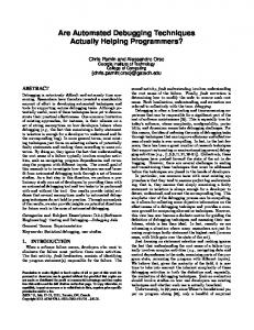
Fig. 1.

Automated post-silicon debugging of design bugs

II. AUTOMATED P OST-S ILICON D EBUGGING OF D ESIGN B UGS For post-silicon debugging usually there are three main components: specification, design, and chip. Specification as a golden model can be a formal specification or a high level simulation model or a testbench. The specification is used for creating the expected correct output of a trace in the debugging process. A design can be a circuit which is represented at Register Transfer Level (RTL) by Hardware Description Languages (HDL). After that, logic synthesis generates the gate level design, and the place-and-route process creates the transistor level design for chip manufacturing. After manufacturing the chip, post-silicon verification is started by running a test program, such as an end-user application or functional tests. In this case, signal traces are stored in trace buffers. Then, a specification is used to validate the stored traces. After detecting an inconsistency between the recorded traces and the specification, this inconsistency is returned as a counterexample. Then, post-silicon debugging starts to localize the bug. Figure 1 shows our overall approach which consists of four steps. These steps are analysis of trace buffer data, modelbased diagnosis (debugging), diagnostic trace generation, and diagnostic trace validation. At the first step, trace buffer data

om

...

... Design

Trace Buffer

...

Design

Control Logic

o1

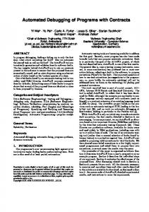
Fig. 2.

Hardware structure

which is obtained after running a test program on the chip should be analyzed and compared with the expected correct outputs obtained from the specification. If there is an inconsistency between trace data and golden data, this inconsistency or erroneous behavior is represented as a counterexample to be used for debugging. The second step of the approach is debugging. Different techniques have been proposed for automated debugging which rely on simulation, Binary Decision Diagrams (BDD), and Boolean Satisfiablity (SAT) [12]. Among these techniques SAT-based debugging [13] as an effective approach to modelbased diagnosis [14] has been shown to outperform previously proposed simulation-based and BDD-based techniques by orders of magnitude in certain cases [12]. In SAT-based debugging, the circuit is first enhanced with a correction model by adding a multiplexer at the output of each component. If the correction model is inactive, the circuit behaves according to its implementation. If the correction model is active, the output of a component may be replaced with a value for correcting the erroneous behavior [9]. The result of SAT-based debugging is a set of fault candidates. Each fault candidate is a potential source of a bug, i.e. a component of the circuit that can be modified to correct the erroneous behavior. In the first iteration SAT-based debugging starts by calculating fault candidates for the initial counterexamples. The third step of the approach, called diagnostic trace generation in Figure 1, is responsible to generate diagnostic traces which may further reduce the number of fault candidates. The inputs of this step include the faulty design and the set of fault candidates. This step generates diagnostic traces by heuristic methods presented in [11]. As a high quality counterexample aims at reducing the number of fault candidates effectively, each diagnostic trace activates a small number of fault candidates and observes their behavior on outputs. Therefore, the counterexamples derived from diagnostic traces are likely to reduce the number of fault candidates.

TABLE I D IAGNOSIS ACCURACY, T IME , AND M EMORY Characteristics of Benchmarks Circuit

#C

Initial Results #FC

Results after Automation

#CE

#FC

#CE

#Trace

Time

Mem

or1200_alu

436

5

1

3

5

41

24.6

54

or1200_ctrl

1865

7

6

7

13

12

3035.1

2332

or1200_genpc

732

20

3

12

8

296

880.8

1154

or1200_if

463

5

3

1

9

6

123.6

652

or1200_lsu

793

3

2

2

9

10

294.7

1163

or1200_operandmuxes

376

11

3

7

8

62

165.1

330

or1200_wbmux

278

7

10

7

15

13

94.2

865

In the step of diagnostic trace validation, diagnostic traces are validated by the specification, because it is not guaranteed that the diagnostic traces really create erroneous output responses in the design. A diagnostic trace which creates erroneous output behavior is a counterexample. The new counterexmples created by the diagnostic traces discriminate the behavior of fault candidates and explain the erroneous behavior of fault candidates for a designer more precisely. If there is no new counterexample, the algorithm returns to the third step for generating more diagnostic traces. By creating the new counterexamples, debugging is iterated to likely increase the diagnosis accuracy with the new set of counterexamples. Thus, the automation may decrease the number of fault candidates. Finally, the small set of fault candidates reduced by automation is shown in the schematic view of the circuit, and designer can rectify the bug by only focusing on a small number of fault candidates. A. Hardware Structure Figure 2 shows the hardware structure used to collect initial counterexamples. The hardware structure is based on the trace buffer as a DFD solution. Control logic is responsible to detect trigger conditions so it can determine when and which data signals will be sampled in the trace buffer. The trigger conditions can be based on time, event, or a mixture of both. The control logic tries to sample signals in a way that the best verification coverage is obtained. For verifying the trace buffer data after running a test program, some inputs, outputs and internal states of the circuit need to be stored in the trace buffer. The signals that need to be sampled at the same time should have independent entries to the trace buffer. The control logic may divide the trace buffer into multiple segments [15]. These segments may belong to signals within different entities or signals related to different events. Also segmentation may be based on the sampling period [8]. For example a trace buffer can have two segments, the first segment for samples from clock cycle 100 to 500, the second segment for samples from clock cycle 800 to 1200. Also the control logic can control the trace buffer as a circular buffer [3]. In this case, information related to the last events can be recovered from the trace buffer. After finishing the test

program or detecting an error, the control logic serializes the content of the trace buffer and sends it back to the off-chip debugger software via a low-bandwidth interface such as JTAG [15]. This data constitutes the initial counterexamples. III. E XPERIMENTAL R ESULTS This section evaluates our approach empirically with respect to diagnosis accuracy, time, and memory. The hardware structure is written at RTL with Verilog hardware description language. The experiments are run on the modules of the OpenRISC CPU from OpenCores [16]. A matrix multiplication program is used as a test program to be run by OpenRISC in the ModelSim environment. The experiments are executed for each module independently. For each experiment, a random single logic bug is inserted into the RTL code. The logic bugs constitute the largest fraction of the design bugs [17] where the design bugs are classified into the logic bugs, algorithmic bugs, and timing bugs. The trace data related to a time window is recorded in the trace buffer of the corresponding module. The time window is set to be 8 cycles. Each window contains initial states at the first step of the window, inputs, and output results at the end of the window. The size of the trace buffer is different for different modules, but the maximum size is assumed to be 8K × 32 bits. For specification, we use the Verilog modules as a black box module giving access only to module inputs, module outputs, and some of the internal registers (states) which would be available in a high level specification, too. For each time window, the recorded initial states and inputs are applied to the RTL design. Then, output results are compared to the output results of the corresponding window in the trace buffer to detect inconsistencies and to constitute initial counterexamples. After having initial counterexamples, the RTL design is unrolled for 8 time steps for debugging. The techniques described in the paper are implemented using C++ in the WoLFram environment [18]. The visualization is performed by RTLvision PRO [19]. Table I presents the experimental results with respect to the diagnosis accuracy, time, and memory. The first and second

Fig. 3.

Initial fault candidates

columns show the module name and the total number of components (#C) considered for SAT-based debugging. The third and fourth columns present the debugging result in the first session when debugging tries to find the potential number of fault candidates (#F C) with the initial counterexamples (#CE). Columns 5-7 show the result when the heuristic method is used for generating the diagnostic traces. The final number of fault candidates found by debugging on all available counterexamples is presented in column 5. The total number of counterexamples (initial counterexamples + created counterexamples by diagnostic traces) is presented in column 6. Column 7 presents the number of diagnostic traces generated by the heuristic method (#T race). Columns 8 and 9 show the required run time (T ime), and the maximum memory consumption (M em). Run time is measured in CPU seconds, and the memory consumption is measured in MB. Consider or1200_alu; trace analysis leads to one counterexample. Debugging finds five fault candidates corresponding to the initial counterexample. Then diagnostic trace generation starts. The process yields four new counterexamples. Finally five counterexamples (one initial counterexample + four new counterexamples) increase the diagnosis accuracy, i.e., decrease the number of fault candidates to three. Also for or1200_genpc, or1200_if , or1200_lsu, and or1200_operandmuxes, the new counterexamples created by diagnostic traces increase the diagnosis accuracy. Figure 3 shows the initial fault candidates for or1200_if . Firstly debugging finds five fault candidates corresponding to the three initial counterexamples. The fault candidates are highlighted with red color. Also the sections of code related to fault candidates are shown. After automation and by creating

the new counterexamples, the number of fault candidates decreases. Figure 4 shows the schematic view of the circuit and its related code after automated debugging. Therefore the designer focuses on a small set of fault candidates and can rectify the bug easily. This reduces the overall development time significantly. IV. C ONCLUSION This paper presented an approach for automating postsilicon debugging when some design bugs escape the presilicon verification and slip into the silicon. The approach integrates four main steps. These steps are data analysis of trace buffer, model-based diagnosis, diagnostic trace generation, and diagnostic trace validation. Then by iterating model-based diagnosis and counterexample generation, diagnosis accuracy increases and post-silicon debug time decreases. R EFERENCES [1] M. Abramovici, P. Bradley, K. Dwarakanath, P. Levin, G. Memmi, and D. Miller, “A reconfigurable design-for-debug infrastructure for SoCs,” in Design Automation Conf., 2006, pp. 7–12. [2] K.-H. Chang, I. L. Markov, and V. Bertacco, “Automating post-silicon debugging and repair,” in Int’l Conf. on CAD, 2007, pp. 91–98. [3] S.-B. Park, T. Hong, and S. Mitra, “Post-silicon bug localization in processors using instruction footprint recording and analysis (IFRA),” IEEE Trans. on CAD, vol. 28, no. 10, pp. 1545–1558, 2009. [4] A. Hopkins and K. McDonald-Maier, “Debug support for complex systems-on-chip: a review,” Proc. of Computers and Digital Techniques, vol. 153, no. 4, pp. 197–207, 2006. [5] B. Vermeulen, T. Waayers, and S. Bakker, “IEEE 1149.1-compliant access architecture for multiple core debug on digital system chips,” in Int’l Test Conf., 2002, pp. 55–63. [6] J.-S. Yang and N. A. Touba, “Expanding trace buffer observation window for in-system silicon debug through selective capture,” in VLSI Test Symp., 2008, pp. 345–351.

Fig. 4.

Fault candidates after automation

[7] Y. Lee, T. Matsumoto, and M. Fujita, “On-chip dynamic signal sequence slicing for efficient post-silicon debugging,” in ASP Design Automation Conf., 2011, pp. 719–724. [8] Y.-S. Yang, N. Nicolici, and A. G. Veneris, “Automated data analysis solutions to silicon debug,” in Design, Automation and Test in Europe, 2009, pp. 982–987. [9] A. Smith, A. Veneris, M. F. Ali, and A. Viglas, “Fault diagnosis and logic debugging using boolean satisfiability,” IEEE Trans. on CAD, vol. 24, no. 10, pp. 1606–1621, 2005. [10] A. Sülflow, G. Fey, and R. Drechsler, “Using QBF to increase accuracy of SAT-based debugging,” in IEEE International Symposium on Circuits and Systems, 2010, pp. 641–644. [11] M. Dehbashi, A. Sülflow, and G. Fey, “Automated design debugging in a testbench-based verification environment,” in Euromicro Conference on Digital System Design (DSD), 2011. [12] A. G. Veneris, B. Keng, and S. Safarpour, “From RTL to silicon: The case for automated debug,” in ASP Design Automation Conf., 2011, pp. 306–310.

[13] G. Fey, S. Staber, R. Bloem, and R. Drechsler, “Automatic fault localization for property checking,” IEEE Trans. on CAD, vol. 27, no. 6, pp. 1138–1149, 2008. [14] R. Reiter, “A theory of diagnosis from first principles,” Artificial Intelligence, vol. 32, pp. 57–95, 1987. [15] E. Anis and N. Nicolici, “Low cost debug architecture using lossy compression for silicon debug,” in Design, Automation and Test in Europe, 2007, pp. 1–6. [16] OpenCores, http://www.opencores.org. [17] K. Constantinides, O. Mutlu, and T. M. Austin, “Online design bug detection: RTL analysis, flexible mechanisms, and evaluation,” in International Symposium on Microarchitecture (MICRO), 2008, pp. 282–293. [18] A. Sülflow, U. Kühne, G. Fey, D. Große, and R. Drechsler, “WoLFram – a word level framework for formal verification,” in IEEE/IFIP Int’l Symposium on Rapid System Prototyping (RSP), 2009. [19] RTLvision PRO, Concept Engineering GmbH, http://www.concept.de.