Hindawi Publishing Corporation Modelling and Simulation in Engineering Volume 2016, Article ID 5309348, 15 pages http://dx.doi.org/10.1155/2016/5309348
Research Article Automated Search-Based Robustness Testing for Autonomous Vehicle Software Kevin M. Betts1 and Mikel D. Petty2 1
Leidos Inc., Huntsville, AL 35806, USA University of Alabama in Huntsville, Huntsville, AL 35899, USA
2
Correspondence should be addressed to Mikel D. Petty;
[email protected] Received 28 April 2016; Revised 4 July 2016; Accepted 10 July 2016 Academic Editor: Min-Chie Chiu Copyright © 2016 K. M. Betts and M. D. Petty. This is an open access article distributed under the Creative Commons Attribution License, which permits unrestricted use, distribution, and reproduction in any medium, provided the original work is properly cited. Autonomous systems must successfully operate in complex time-varying spatial environments even when dealing with system faults that may occur during a mission. Consequently, evaluating the robustness, or ability to operate correctly under unexpected conditions, of autonomous vehicle control software is an increasingly important issue in software testing. New methods to automatically generate test cases for robustness testing of autonomous vehicle control software in closed-loop simulation are needed. Search-based testing techniques were used to automatically generate test cases, consisting of initial conditions and fault sequences, intended to challenge the control software more than test cases generated using current methods. Two different search-based testing methods, genetic algorithms and surrogate-based optimization, were used to generate test cases for a simulated unmanned aerial vehicle attempting to fly through an entryway. The effectiveness of the search-based methods in generating challenging test cases was compared to both a truth reference (full combinatorial testing) and the method most commonly used today (Monte Carlo testing). The search-based testing techniques demonstrated better performance than Monte Carlo testing for both of the test case generation performance metrics: (1) finding the single most challenging test case and (2) finding the set of fifty test cases with the highest mean degree of challenge.
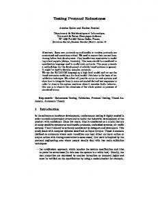
1. Introduction The use of autonomous systems is growing across many areas of society, with further increases planned in the next decade [1]. While originally used predominantly in the military domain, the use of autonomous systems has increased in the commercial marketspace as well. Figure 1 shows an example of two different autonomous systems under development: the Google self-driving car [2] and autonomous unmanned aerial vehicle (UAV) delivery drones. The expanded uses of autonomous vehicles will require increased software functionality including higher-level reasoning capabilities, improved sensing and data fusion capabilities, and more robust control algorithms [3]. Autonomous systems will be expected to complete their missions under both nominal and off-nominal conditions, as there will be financial impacts and possibly safety-of-life concerns if the systems cannot perform as expected across a wide range of operating conditions.
Testing the software that controls autonomous vehicles operating in complex dynamic environments is a challenging task. Due to cost and time considerations, software testing with digital models is used to augment real-world tests run with the actual autonomous vehicle. Model-based testing methods are frequently used for autonomous vehicle software testing, wherein an executable version of the vehicle software under test (SuT) and a simulation of the vehicle and operating environment (known as the Simulation Test Harness) are both developed in the initial stages of the project to provide early opportunities for integration and closed-loop testing. There are a wide number of variables that influence system performance for a particular mission, including variations in the weather, spatial environment, and hardware component performance. The system will also be required to complete its mission (or safely abort) when faults such as hardware malfunctions or weather anomalies occur. The fault occurrence time for a specific fault is the time when
2
Modelling and Simulation in Engineering
(a)
(b)
Figure 1: Photographs of (a) Google self-driving car (image source: Wikipedia Commons. Author: Mark Dolinar. Used under the Creative Commons Attribution-Share Alike 2.0 Generic license) and (b) autonomous UAV (image source: Wikipedia Commons. Author: Miki Yoshihito. Used under the Creative Commons Attribution-Share Alike 2.0 Generic license).
the fault occurs during the mission or a simulation of it. Testing autonomous vehicles requires assessing both different combinations of faults that may occur together as well as different fault occurrence times for those faults. One important objective for testers of autonomous vehicle software is to generate an adequate set of test cases to assess overall system robustness. Robustness testing is defined as a testing methodology to detect the vulnerabilities of a component under unexpected inputs or in a stressful environment [4]. It was introduced in Department of Defense programs to focus on early identification of test cases that cause failures [5]. A test case in this context is defined as the initial conditions for the mission as well as specific system faults and the times when they occur. Robustness testing prioritizes the identification and use of challenging test cases that are more likely to reveal conditions that cause performance requirements to not be met. For real-world autonomous systems, it is not possible to test all combinations of initial conditions and fault sequences. The multidimensional test space is too large to combinatorially generate and execute all possible test cases in the time allocated for software testing. Therefore, given a SuT that must control the vehicle and a Simulation Test Harness to provide the sensor inputs to the SuT and to act on the SuT’s commands, the tester must identify and prioritize the most challenging sets of valid test case conditions. The remainder of this paper is organized as follows. Prior related research is summarized in Section 2. Section 3 details the technical approach and experimental set-up for this research. The results of the experiments comparing the automated test case generation methods are reported in Section 4. Finally, the conclusions are given and possible future work is identified in Section 5.
2. Background This section provides relevant background information on the overlapping disciplines related to this research. Section 2.1 discusses the model-based testing process used with autonomous vehicle software. Section 2.2 describes methods typically used for automated test generation (ATG), while
Section 2.3 discusses search-based testing (SBT), a particular subclass of ATG, in more detail. Previous attempts to use SBT methods for autonomous vehicle software testing are presented in Section 2.4. 2.1. Model-Based Testing for Autonomous Vehicle Software. Autonomous vehicle software is typically assessed using model-based testing methods prior to field deployment. Model-based testing connects the autonomous vehicle SuT with a Simulation Test Harness that is used to test closed-loop interactions between the SuT and the vehicle in the context of the intended operating environment. The Simulation Test Harness models the behavior of the vehicle and its associated hardware being controlled by the SuT as well as the vehicle’s external environment. Because the SuT for an autonomous system must make decisions based on sensed data from the environment, it requires a closed-loop test capability to realistically assess software performance. The SuT can begin as an executable model of the software and later be replaced with more mature code instantiations. Figure 2 shows a progression through the software development and test cycle using model-based testing principles. The need to test the SuT exhaustively in simulation throughout the development cycle to emulate conditions that will not be field tested with the real system was emphasized in [7]. Software integration begins with Model-in-the-Loop (MIL) and Software-in-the-Loop (SIL) testing run in alldigital environments. Later, the software is ported to run on the vehicle computer for Processor-in-the-Loop (PIL) testing. The system progresses to hardware-in-the-loop (HIL) testing where sensors and actuator models are replaced by hardware components. An emphasis on generating challenging test cases early in this process can be highly beneficial, as changes to the SuT are much less costly and time consuming to make during the early phases of the project (MIL and SIL). A Simulation Test Harness for a complex system typically has system initial conditions that can vary across scenarios. Frequently, these initial conditions are stochastic in nature and can vary from run to run. They can emulate differences in behavior across individual hardware components that may be present in a specific vehicle. They also represent
Modelling and Simulation in Engineering
3
Requirements System test
System design Controller design MIL simulation
Calibration
Controller test
Software design
HIL simulation
Integration
Code building process
PIL simulation
SIL simulation
Figure 2: Model-based testing process (adapted from [6]).
environmental variables such as wind speed and direction, air density, and precipitation conditions. Another important capability of the Simulation Test Harness is the ability to simulate system faults or failure modes that may occur in the real world and that the system is designed to respond to with appropriate behavior. Fault insertion is the method of injecting or inserting a fault into the Simulation Test Harness at a specified time, which triggers changes in the simulated behavior of the system. Examples of possible faults include hardware (obscured sensor lens or stuck actuator motor) as well as environment effects (strong wind gusts). The SuT contains software that must command the appropriate response when a fault occurs, which sometimes requires initial evaluation and diagnosis that the problem occurred to ensure the proper response is commanded. Faults can often occur within wide ranges of time during the mission, and the Simulation Test Harness must be capable of inserting the specified fault and correctly propagating the effects through the rest of the simulation at any given time specified for the fault insertion. 2.2. Automated Test Generation. Because a large number of test cases are desired to test autonomous vehicle software robustness, ATG methods can be used to significantly augment the number of test cases that can be developed manually. As the name implies, ATG is the ability to automatically generate test cases to be used for exercising software code to evaluate its suitability for its intended purpose. Software testing can take up to 50% of the overall software development budget [8], and manual test case development by subject matter experts is both expensive and time consuming. Therefore, there has been increased focus on ATG programs in the past 15 years. The most complete form of ATG software robustness testing is full combinatorial testing of all possible input parameters. For simple software units where a small number of input values have been discretized into a small set of specific enumerations, it may be possible to test all possible combinations of input values. Combinatorial testing was performed in [9] to support testing of a launch vehicle failure detection, diagnostics, and response system using a simplified vehicle simulation. All possible test cases were generated by
varying model input variables (setting variables to maximum, nominal, or minimum values) and failure mode insertions (with fault occurrence times restricted to occur at specific points in time rather than all possible time). However, for most real-world systems, it is highly unlikely that all combinations of inputs can be tested in a realistic amount of time due to the exponential growth of the test space as the number of initial conditions, faults, and possible fault occurrence time increase. Figure 3 illustrates this effect. The dots scattered around the coordinate axes in the diagram on the left represent possible initial conditions for the mission. The fault insertion portion of the test case comprises the specific faults selected and the specific times when those faults are activated, generating a large number of possible fault cases for a single set of initial conditions. For each possible initial condition, each of these fault profiles could be activated. Combining initial condition generation with fault insertion is what can lead to a truly large test space for the ATG algorithm. The inability to test all possible combinations motivates a range of approaches for selecting and prioritizing test cases to be run. One approach frequently used is to leverage Design of Experiment (DoE) principles originally developed in the statistics and operations research communities. DoE is a method of generating a series of tests in which purposeful changes are made to the system input variables and the effects on response variables are measured. DoE principles can be used to analyze simulations with large numbers of input and output variables [10, 11]. Fractional factorial experiments can be used when full combinatorial testing is not feasible due to the large number of system input variables. Results from fractional factorial designs enable system designers to understand the main effects and low-order interactions of simulation parameters with significantly fewer runs than would otherwise be required to obtain full observability into all higher order interaction terms. Monte Carlo (MC) testing is the ATG method most commonly used today to assess autonomous vehicle software robustness [12–16]. The initial conditions, system faults, and fault insertion times are generated randomly in MC testing using suitable probability distributions. This process is repeated (changing the input parameters for every new
4
Modelling and Simulation in Engineering z-axis
Fault m inserted
Fault m ··· Fault 3 Fault 2 y-axis
Fault 3 inserted
Fault 2 inserted
Fault 1 Time Fault m inserted
Fault m ··· x-axis
Fault 3 Fault 2
Fault 3 inserted Fault 1 inserted
Fault 1
Time Fault m inserted
Fault m ··· Fault 3 Fault 2 Fault 1
Fault 1 inserted
Fault 2 inserted Time
···
Figure 3: Example of multiple fault injection timelines occurring for a single initial condition.
run) until the specified number of runs is completed. The system performance metrics (now represented as stochastic variables) can be examined to determine compliance with system requirements. 2.3. Search-Based Testing. SBT is a subdiscipline within ATG that uses optimization techniques to generate challenging test cases. Approaches used in SBT include metaheuristic algorithms, branch-and-bound algorithms, and mixed integer linear programming [17]. In this research, two different SBT methods were evaluated: (1) genetic algorithms (GAs) and (2) surrogate-based optimization (SBO). The following paragraphs describe these methods in more detail. 2.3.1. Genetic Algorithms. GAs are a specific type of metaheuristic search algorithm that are frequently applied to global optimization problems with many input variables. Metaheuristic algorithms are used to solve problems with minimal assumptions about the form of the solution before beginning the optimization process. For real-world problems with a large number of possible input variable values, it is frequently impossible to guarantee finding the globally optimal solution in finite time. Metaheuristic algorithms do not guarantee the optimal solution but are typically quick to execute and attempt to search widely across the solution state space to identify and promote particularly promising input variable combinations. The GA is a popular metaheuristic algorithm that uses a population of candidate solutions iterated (evolved) over time in an attempt to improve the value of the defined fitness functions [18]. GAs typically
require encoding the solution space as a binary string of ones and zeros, though other encoding schemes can be used [19]. Problem constraints (such as input minimum and maximum bounds) are enforced during candidate creation to ensure that invalid solutions are not attempted. After each iteration (also known as a generation), promising solutions are paired to produce new solutions by combining elements of each candidate solution (also known as breeding). Successful candidate solutions can also be mutated (random flipping of the elements of the solution) in an attempt to find other nearby solutions which may further improve the fitness function. This process continues over time until a maximum number of iterations are reached or a predefined fitness objective value is achieved. GAs have a long history of use for SBT applications. A systematic review of SBT for finding test cases that will cause the system to no longer function as expected is given in [20]. Of the 15 examples of past work focused on generation of challenging test cases, GAs were used in 14, with simulated annealing used in the other. GAs were also used for test case generation for simple and complex software units in [21]. For simple function tests, the GA equaled or outperformed Monte Carlo test generation at finding challenging test cases for every function, with performance improvements as large as 35.7%. However, none of the applications in [20] or [21] focused on closed-loop model-based testing with interactions between the SuT and a Simulation Test Harness. 2.3.2. Surrogate-Based Optimization. SBO is an optimization technique that creates a surrogate model (or metamodel)
Modelling and Simulation in Engineering that is used in place of a computationally expensive objective function (often a simulation of a physics-based model) when performing certain optimization calculations. The goal of SBO is to minimize the number of required executions of the expensive objective function while still being able to perform a global search. The results of the surrogate model predictions are used to carefully select the next point for objective function evaluation. A variety of surrogate models have been used in SBO applications, including polynomial, radial basis functions, and Kriging models [22]. SBO has more typically been used in the design phase of system development rather than the test phase. The use of surrogate models in the design optimization problem is discussed in [23]. Because it is often not computationally feasible to directly optimize a complex system design using a large number of high-fidelity simulation runs, developing response surfaces based on surrogate models helps the designer attempt to jointly optimize several design criteria in the available time allotted to system design. The reasons why SBO techniques may have been used less frequently for test applications than for design are discussed in [24]. Many SBT applications focus on direct testing of the SuT, that is, direct manipulation of the input vector for the SuT. For most of these applications, the evaluation of the objective function is relatively inexpensive because it does not require executing a simulation [25]. This is in contrast to indirect SBT testing, such as autonomous vehicle closed-loop model-based testing, where the test case parameters are generated to change the behavior of the Simulation Test Harness. The Simulation Test Harness then generates inputs for the SuT and reacts to the commands from the SuT. Each run of the Simulation Test Harness can be computationally expensive, thus motivating optimization techniques that attempt to limit the number of required simulation executions. Therefore, SBO techniques are much more relevant to indirect search-based test applications such as autonomous vehicle software test case generation. 2.4. Previous Uses of Search-Based Testing for Autonomous Software Testing. While there has been a large amount of work performed in both model-based testing and SBT areas, there are only a small number of examples of using these techniques together—that is, the use of SBT principles applied to closed-loop model-based testing. One prominent example in this field is the TestWeaver software package [26–30]. Test case generation is described as playing a game against the SuT with the intention to drive it to a state that violates its specifications. If the test algorithm is able to successfully generate such a test case, it has “won” the game. TestWeaver is capable of setting initial conditions as well as inducing faults; however, the simultaneous optimization of fault combinations and occurrence times across the simulation is not discussed. The branch search process is described as being similar to the minimax artificial intelligence algorithm sometimes used in chess-playing programs. TestWeaver was used in the testing of several automobile subcomponents, including dual-clutch transmission systems, chassis control systems, and crosswind stabilization components. There are
5 no performance comparisons to other ATG testing methods or to a truth reference for any of the examples given. GAs are used to find rule-based fault conditions that cause failures in autonomous vehicle controllers in [31]. The goal is to find “combinations of faults that produce noteworthy performance by the vehicle controller” using closed-loop testing methods. Results are shown for fault insertions that occur for a nominal set of initial conditions, but no test cases were derived that simultaneously optimized initial conditions and fault combinations. The GA test case generation results are not compared to alternate ATG techniques or to a truth reference. In summary, there are no examples in the literature that attempt to perform simultaneous SBT optimization of initial conditions, fault combinations, and fault occurrence times for closed-loop model-based testing applications.
3. Methods In order to quantify the performance of SBT algorithms when used in autonomous vehicle model-based testing applications, SBT performance was compared to the performance of the method most commonly used today (MC testing) as well as the theoretical upper bound of performance for this problem (as determined by full combinatorial testing). To support these objectives, a medium complexity Simulation Test Harness has been developed. The Simulation Test Harness was intentionally designed to include sufficient features and variables to support a meaningful comparison of the test case generation methods without being so complex as to preclude the generation of a full combinatorial set of test cases to be used for comparison. The key feature of this test set-up is that the total number of input variables (initial conditions and fault parameters) was small enough that complete combinatorial testing of the system was feasible but large enough to reveal performance differences between the ATG methods that were compared. Being able to evaluate each possible combination of input conditions made it possible to enumerate a full ranking of the maximum error for all possible test cases. The ATG algorithms (MC and SBT) were constrained to perform significantly fewer simulation runs than the full combinatorial testing, thus enabling evaluation of their effectiveness and efficiency relative to a known truth baseline. It is assumed that, for complex real-world systems, the execution of the high-fidelity simulation interacting with the vehicle control software will be very computationally expensive, thus limiting the number of simulation executions that the tester will be able to execute while generating test cases. Therefore, in this research, the SBT algorithms were constrained to run only a fraction of the total possible combinations, ranging from 0.03% in the most limiting trial up to 1.27% for the trial with the most allowed simulation executions. The problem for this research was testing UAV flight control software attempting to steer a small UAV quadcopter through a 10 m entryway. As seen in Figure 4, the objective of the UAV flight control software is to guide the UAV through the middle of the entryway; that is, to minimize the lateral
6
Modelling and Simulation in Engineering
Wall
Intended flight path through entryway
Wall
5m
xlongitudinal xlateral UAV Top down view
Figure 4: Depiction of the UAV flight control software test problem.
deviation from the intended flight path so as to provide maximum margin while passing through the entryway. The development of UAV control software for flight through complex spatial environments is an active area of research, as demonstrated by the DARPA Fast Lightweight Autonomy (FLA) program [32]. The FLA program focuses on highspeed flight in cluttered environments including transitions from outdoor to indoor operations. In order to assess the UAV flight control software’s robustness, an objective of the software testing process is to define test cases that will maximize the test case degree of challenge, in this case, the lateral deviation of the UAV. For this particular example problem, the system can pass through the entryway if the lateral deviation is no more than ±5 meters of the intended flight path, a straight line passing the center of the entryway. If the UAV can successfully pass through the entryway with the required success rate over the most challenging set of test cases that can be generated, the UAV development team will have increased confidence the system is ready for the actual flight test phase. 3.1. Test Architecture. Figure 5 provides an overview of the overall test architecture. The UAV flight control software is the SuT for this system. It receives sensor feedback about the external environment and issues actuator commands to attempt to correctly steer the UAV. The Simulation Test Harness is responsible for simulating the UAV hardware (including sensors and actuators), the external environment, and the equations of motion of the UAV. The ATG algorithm generates test cases in an attempt to challenge the SuT and receives feedback from the Simulation Test Harness in the form of the final lateral deviation for each generated test case. The final output of the ATG algorithm at the completion of its execution is a ranked set of the generated test cases. The following sections describe each of the primary components of the system in more detail. 3.2. Simulation Test Harness. Figure 6 is a block diagram that includes the subcomponents of the Simulation Test Harness. The Rotor Actuator model receives the actuator command from the flight control software and produces an achieved lateral force. The equations of motion generate the
position and velocity state derivatives of the UAV based on the UAV mass properties as well as the sum of forces acting on the vehicle. The integrator module uses Euler forward integration to transform the state derivatives into the position and velocity true vehicle state. For this example problem, the equations of motion operate in two dimensions; it is assumed that a separate vertical controller operates to stabilize the altitude of the vehicle within the desired operating band. Finally, the Lateral Sensor model observes the true state of the vehicle and generates an estimate of the lateral position as sensor feedback for the flight control software. Both the Rotor Actuator model and the Lateral Sensor model have error characteristics. The achieved lateral force generated by the Rotor Actuator model and the sensed lateral position observed by the Lateral Sensor are subject to error terms due to hardware imperfections that prevent them from generating perfect output values based on their inputs. Each test case for evaluating the flight control software consists of six initial condition variables and three faults. The six initial conditions are lateral position, lateral velocity, actuator bias, actuator scale factor, sensor bias, and sensor longitudinal scale factor. The three faults that can occur are a stuck actuator, a sensor multipath error, and an intermittent wind gust. A fault may occur during a single time step of the simulation (between the first and last time steps), or it may occur not at all in a given test case. The state variables of the motion model are 𝑥 = {𝑥longitudinal 𝑥lateral Vlongitudinal Vlateral }𝑇 , where 𝑥longitudinal and 𝑥lateral are the UAV position states along the longitudinal and lateral axes as defined by the intended flight path through the center of the entryway, and Vlongitudinal and Vlateral are the velocity states along these same axes. Equation (1) provides the UAV equations of motion in state space form: 0 0 1 0 [ ] [ [0 0 0 1] [ ]𝑥 + [ 𝑥̇ = [ [0 0 0 0] [ [ ] [ [0 0 0 0]
0 0 0
] ] ], ] ]
(1)
[ 𝑤gust + 𝑓act ]
where 𝑥̇ is the state vector derivatives, 𝑥 is the state vector, 𝑤gust is the force imparted by a wind gust that can occur when the wind fault variable is present, and 𝑓act is the lateral force applied by the Rotor Actuator. 𝑓act is composed of the following terms: {𝑓cmd + 𝑓bias + 𝑓sf ∗ 𝑓cmd 𝑓act = { 𝑓 { prev
if 𝑓stuck = 0 if 𝑓stuck = 1,
(2)
where 𝑓cmd is the force commanded by the flight control software, 𝑓bias is the lateral actuator bias, 𝑓sf is the lateral actuator scale factor, and 𝑓stuck is a binary fault variable indicating if the actuator is unable to respond at a given time step. The model is executed for five seconds, and a time step of 1 second is used. Note that a higher fidelity dynamics model would normally use a much smaller integration step
Modelling and Simulation in Engineering
7
Set of possible initial condition values
Automated test generation algorithm
Set of possible faults and occurrence times
Final lateral deviation
Generated test case
Flight control software
Actuator command
Ranked set of generated test cases
Simulation Test Harness
Sensor feedback
Figure 5: Automated test generation architecture for UAV flight control software testing.
Environment model
Flight control software
Actuator command
Rotor actuator
Simulation test harness
Wind gust force
Achieved lateral force
Sensor Feedback
Equations of motion
State vector derivatives
Integrator
True vehicle state
Lateral sensor
Figure 6: Block diagram of the UAV Simulation Test Harness.
to capture high-frequency dynamic effects. For this example, a coarse time step is used in order to limit the total number of fault insertion points in the model, thus enabling the generation of a truth reference through full combinatorial testing of all possible test cases. This truth reference is used to assess the performance of the test case generation algorithms being developed. The Lateral Sensor model is composed of the following terms: 0 [ ] [1] ] 𝑦=[ [ 0 ] 𝑥 + 𝑠bias + 𝑠long sf ∗ (5 − 𝑥longitudinal ) [ ]
(3)
[0] + 𝑠multipath , where 𝑦 is the sensor output (estimated lateral position), 𝑠bias is the sensor bias term, 𝑠long sf is the longitudinal scale factor, and 𝑠multipath is the multipath error that is present when the multipath fault variable is triggered. For the error contribution of 𝑠long sf term, the error is largest when the UAV is farthest away from the entryway (𝑥longitudinal = 0) and decreases to zero as the UAV arrives at the entryway (𝑥longitudinal = 5).
3.3. Flight Control Software. The SuT for this research problem is the flight control software of the UAV. Its objective is to minimize the lateral deviation relative to the intended flight path while the vehicle is passing through the entryway. The flight control software accepts as input the imperfect Lateral Sensor model estimate of the lateral position and produces as output a command to the UAV Rotor Actuator. As described above, the force actuator is incapable of perfectly implementing the commanded value from the flight control software. Equation (4) defines the proportional control law used by the flight control software to reduce the lateral deviation of the UAV: {max {−1.3 ∗ 𝑥lateral , −1.5} 𝑓cmd = { min {−1.3 ∗ 𝑥lateral , 1.5} {
if 𝑥lateral > 0 if 𝑥lateral < 0,
(4)
where 𝑓cmd is the desired control force commanded by the flight control software. Note that the controller has a maximum possible force it can generate in a given time step, thus leading to the max and min operations in the above equations depending on the direction of the commanded control force. 3.4. Automated Test Generation. The ATG algorithms are responsible for automatically generating the test cases used to assess UAV flight control software performance. Three ATG
8 techniques will be analyzed and compared: MC, GA, and SBO. 3.4.1. Monte Carlo Testing. Test cases for the MC testing were generated randomly using uniform probability distributions. For each of the six initial condition variables, each of the three possible values (minimum, midpoint, maximum) was equally likely, and for each of the three fault variables, each of the six possible values (occurring at 1, 2, 3, 4, or 5 seconds, or not occurring) were equally likely. 3.4.2. Genetic Algorithm. The GA is a good metaheuristic algorithm candidate for this problem due to its potential to perform well for both test case generation performance metrics: finding the single most challenging test case (fittest member of the population) as well as generating a set of challenging test cases through the natural evolution of the entire population. The UAV test case generation problem was framed as a discrete optimization problem where the initial conditions could took one of three values and the fault insertion time could take one of six values. The objective of the GA was to find test cases that maximized the final lateral miss deviation. The MATLAB ga function from the Global Optimization Toolbox was used to perform the optimization [33]. For each trial, the maximum number of allowed executions of the Simulation Test Harness was defined and used to determine when to terminate execution of the GA. The number of allowed executions for each trial was then divided into a total population size (the number of test cases to be evaluated in each generation) and a total number of generations to be evolved. The product of the population size and the number of generations equal the maximum number of allowed executions for a given trial. For this research, population sizes in the range of 5–10% of the maximum number of allowed executions typically gave the best results, resulting in a range of 10–20 generations across the trials. Figure 7 shows the flowchart describing the GA process, with each major step numbered in the upper right corner. The inputs at initialization are the set of possible initial condition values for each variable and the set of possible faults and their possible occurrence times. These inputs define the constraints used to ensure that valid test cases are generated during the ATG process. The final output of the GA at the completion of its execution is a ranked set of the generated test cases, with the test case with the maximum final lateral deviation ranked highest. Step 1 of the GA randomly generates the population of the initial generation of test cases using the constraints on allowable values for initial conditions, faults, and fault occurrence times. Step 2 sends the initial population of generated test cases to the Simulation Test Harness for evaluation. The Simulation Test Harness runs each generated test case in closed-loop fashion with the Flight Control Software. The final lateral deviation is calculated for each generated test case that is evaluated, and this value is sent back to the GA.
Modelling and Simulation in Engineering Step 3 sorts the generated test cases based on the final lateral deviation they produced, with the highest ranked test case being the one that produced the maximum lateral deviation. The GA then evaluates if the stop criteria for the current trial has been met. For this research, the number of Simulation Test Harness Executions performed is compared to the maximum number allowed for the current trial. If the number of allowed executions has not been reached, the GA moves to Step 4 and begins creating the next generation of test cases for evaluation. Step 4 selects the elite member of the previous generation for inclusion as a member of the next generation. For this research, the elite member is the test case with the largest final lateral deviation as calculated by the Simulation Test Harness. The elite member is automatically advanced to next generation of test cases. This ensures that the largest final lateral deviation value for the next generation will always be equal or larger than the previous generation’s maximum value. Step 5 selects parent test cases to be used to produce offspring in the next step of the process. Parent selection uses a weighted random draw where test cases with larger final lateral deviations are more likely to be selected. Step 6 performs the crossover operation using the parents that were selected in Step 5 to create offspring in the form of new test cases that have attributes from both parents. As discussed above, each test case is composed of nine values (six initial conditions and three fault values). The genetic algorithm considers each of these nine entries to be a gene of the parent test case. The crossover process mixes these genes across the two parents. For this research, a scattered crossover function was used. A nine-entry random binary vector is generated, with each entry having a value of 0 or 1. During the crossover operation, the offspring is created by taking the genes from Parent 1 in all cells where the random binary vector has a value of 0 and taking genes from Parent 2 in all cells where the value is 1. This ensures that new offspring are created that combine properties from both parents. Step 7 introduces potential mutations into the population. The mutation process randomly changes gene values to help introduce additional randomness into the search process. Mutation helps the process avoid convergence on local minima due to lack of diversity in the current generation of parents. A random number generator is used to determine if any of the values in the test cases will be changed to a different value. For both the crossover and mutation steps, the input constraints on initial conditions, valid faults, and fault occurrence times are enforced to ensure that only valid test cases are generated. If an invalid test is generated that violates these constraints, the test case is aborted and the process is repeated until a valid test case is generated. Following Step 7, the next generation of test cases is sent to Step 2 for evaluation in the Simulation Test Harness, and the process repeats until the maximum number of allowed evaluations is reached. The final output at termination is the ranked set of all test cases that were generated.
Modelling and Simulation in Engineering
Set of possible initial condition values
Set of possible faults and occurrence times
9
Automated test generation algorithm: genetic algorithm Defines constraints on valid test cases used in steps 1, 6, and 7
Initialize: randomly generate initial population of test cases
1
Send cases to simulation test harness for evaluation
2
Sort test cases based on final lateral deviations
3
Stop criteria?
Yes
Ranked set of generated test cases
No Next gen. of test cases
Select elite members of population
4
Select parents
5
Perform cross-over operation
6
Perform mutation operation
7
Generated test case Flight control software
Actuator command
Simulation Test Harness
Final lateral deviation
Sensor feedback
Figure 7: Flowchart of the genetic algorithm automated test generation algorithm.
3.4.3. Surrogate-Based Optimization. An SBO method based on [34] was used. Figure 8 is a flowchart describing the steps used in the SBO algorithm. As with the GA, the inputs at initialization are the set of possible initial condition values for each variable and the set of possible faults and their valid set of occurrence times. The output at completion of the algorithm is a ranked set of the generated test cases, with the test case with the maximum final lateral deviation ranked highest. Step 1 of the SBO uses Latin Hypercube Sampling based on DoE principles to generate the initial set of test cases. Latin Hypercube Sampling is a form of stratified sampling that attempts to distribute samples evenly across the sample space. For this research, the initial design typically consumed 20–40% of the total available simulation executions for the trail.
Steps 2 and 3 are very similar to the corresponding steps described above for the GA. Generated test cases are sent to the Simulation Test Harness for evaluation, and the generated test cases are sorted based on the final lateral deviation values returned from the Simulation Test Harness. The stop criteria are again evaluated to determine if the total number of allowed Simulation Test Harness Executions has been met or exceeded. If not, the algorithm proceeds with generating the next test case to be evaluated. Step 4 creates a surrogate model for the Simulation Test Harness by fitting a cubic polynomial regression model to the output of all available Simulation Test Harness evaluations. The inputs to the surrogate model are the generated test cases (each comprising values for the six initial condition variables and the three fault variables) that have been evaluated in the
10
Modelling and Simulation in Engineering
Set of possible initial condition values
Set of possible faults and occurrence times
Automated test generation algorithm: surrogate based optimization Defines constraints on valid test cases used in steps 1, 5a, and 5b
1 Initialize: generate initial samples using latin hypercube sampling Send case(s) to simulation test harness for evaluation
Sort test cases based on final lateral deviations
Stop criteria?
2
3
Yes
Ranked set of generated test cases
No 4 Fit polynomial model to Simulation Test Harness results
Generate 5a candidates with local sampling
Generate 5b candidates with global sampling
6 Select best candidate for next Simulation Test Harness evaluation Generated test case Flight control software
Actuator command
Simulation Test Harness
Final lateral deviation
Sensor feedback
Figure 8: Flowchart of the surrogate-based optimization automated test generation algorithm.
Simulation Test Harness. The goal is to create a surrogate model that approximates the final output of the Simulation Test Harness while being much less computationally expensive to evaluate. Steps 5a and 5b use local and global sampling strategies, respectively, to identify potential test cases to evaluate next in the Simulation Test Harness. Because the surrogate model can be executed more quickly than the Simulation Test Harness, it makes sense to evaluate many candidate points with the surrogate model in order to determine the strongest possible candidate for the next Simulation Test Harness execution. In Step 5a, a local sampling algorithm is used to generate 25 new potential test cases. This algorithm adds random local perturbations to the test case with the largest final lateral deviation found to date using the Simulation Test Harness. The surrogate model is then evaluated for each of these
25 potential test cases to estimate the expected final lateral deviation. In Step 5b, a uniform global sampling algorithm is used to attempt to help the algorithm avoid local minima. The state space is uniformly sampled to generate 25 new potential test cases, and again the surrogate model is evaluated for each potential test case. In Step 6, the next Simulation Test Harness candidate test case is selected from the set of 50 potential test cases generated by the local and global sampling algorithms. The selection algorithm uses a weighted calculation that considers both the predicted final lateral deviation based on the surrogate model and how far away in the state space each potential test case is from the test case with the maximum final lateral deviation evaluated so far by the Simulation Test Harness. Test cases that are farther away in the state space are
Modelling and Simulation in Engineering 15 Lateral deviation (m)
rewarded in the selection process to help minimize the risk of being stuck in a local minimum. Once the best candidate is selected in Step 6, it is sent to Step 2 for evaluation in the Simulation Test Harness, and the process begins again. This process continues until the maximum number of allowed Simulation Test Harness evaluations is reached and the algorithm is terminated. The final output at termination is the ranked set of all test cases that were generated.
11
10 5 0 −5 −10 −15
0
1
2
3
5
4
Time (sec)
4. Results The following sections present the results of the research. Section 4.1 describes the test generation performance metrics to be used to evaluate algorithm performance. Section 4.2 provides the results for the three ATG methods tested (MC, GA, and SBO).
Figure 9: Complete time-histories of the UAV flight trajectories for all possible test cases. ×104 3.5 3
4.1.1. Truth Reference Generation. The UAV flight control problem for this research was carefully constrained to make full combinatorial testing possible to enable generation of a truth reference for evaluating ATG algorithm performance. Full combinatorial testing generates the complete set of possible test cases by evaluating all possible combinations of initial conditions and fault occurrence times. In this case, there were six initial condition variables, each of which could have one of three discrete values (minimum, midpoint, and maximum values). Therefore, there are 36 = 729 initial condition combinations that can be tested when no faults are inserted. For a given set of initial conditions, the three fault variables can each take one of six values, inserted at times 1, 2, 3, 4, and 5, or not inserted, giving a total of 63 = 216 fault variations. The total number of possible test cases when initial condition variations and faults are considered simultaneously is therefore 729 ⋅ 216 = 157,464 test cases. Figure 9 shows a plot of the time-history of the UAV trajectories generated for all possible simulation executions. The absolute value of lateral deviation at the end of the simulation (when the UAV is passing through the entryway) is the metric used to assess the test case degree of challenge; larger lateral deviation indicates greater challenge. Figure 10 shows a histogram of these values for all 157,464 possible simulation executions. Of the possible executions, 331 (0.21%) had lateral deviations greater than the requirement of 5 m, while 79 (0.05%) were larger than 6 m and 15 (0.01%) were larger than 7 m. The maximum lateral deviation found was 7.47 m. For more realistic autonomous software testing problems, combinatorial testing is not an option in the time available for testing. For example, for a basic high-fidelity Simulation Test Harness with 20 initial conditions, 10 faults, and an execution time of 15 seconds with a 0.1 second time step,
2.5 Frequency
4.1. Test Generation Performance Metrics. The generation of the truth reference test case rankings for the UAV flight control problem is discussed in Section 4.1.1, while Section 4.1.2 describes the specific test case generation performance metrics used to evaluate ATG algorithm performance.
2 1.5 1 0.5 0
0
1
2 3 4 5 6 Maximum lateral deviation (m)
7
8
Figure 10: Absolute value of the lateral deviations for all possible test cases.
the total possible number of test cases exceeds 1021 . This combinatorial explosion motivates the use of more selective ATG methods that require fewer simulation executions to generate challenging test cases. 4.1.2. Performance Metrics. We evaluate ATG performance for three different algorithms (MC, GA, and SBO) for varying numbers of total allowed simulation executions, as shown in Table 1. The table also expresses the allowed simulation executions for each trail as a percentage of the total possible simulation executions. Each algorithm will be evaluated for two different test case generation performance metrics: (1) the maximum lateral deviation for a single test case and (2) the highest mean lateral deviation value for a set of 50 test cases. These two different performance metrics were selected based on the need to accommodate different test strategies depending on the potential use of the autonomous vehicle. For very expensive autonomous vehicles with large amounts of redundancy (such as a deployed military UAV), it is expected that the system will be able to meet the requirements for almost all possible combinations, so striving to identify the single test case with the largest deviation relative to the
12
Modelling and Simulation in Engineering Table 1: Number of simulation executions allowed for each experimental trial.
Trial Number of simulation executions allowed Percentage of total possible simulation executions
1 50
2 100
3 200
4 500
5 1000
6 2000
0.032%
0.064%
0.127%
0.318%
0.635%
1.270%
Table 2: Maximum lateral deviation (in meters) as a function of simulation executions. 1 50 4.27 3.95 4.76
2 100 4.59 4.33 6.85
requirement is of the most value in order to estimate system robustness to worst case conditions. For less expensive systems such as small commercial UAVs, less redundancy is built into the system because a vehicle failure should not result in loss of life or significant monetary damage. Therefore, the testers are most likely to be interested in generating a wider range of robustness test cases to understand general system reliability across a range of conditions. 4.2. Automated Test Generation Algorithm Evaluation Results. This section presents the ATG results for the two performance metrics for each of the simulation trials, which differed in number of simulation executions. The objective of this research is to determine if the SBT methods (GA and SBO) can generate test cases with equal or higher lateral deviations than MC testing when using the same number of simulation executions. Because random sampling is used in all three ATG algorithms tested, 50 repetitions were conducted for each method for each trial, and the mean value of the parameter over those repetitions is included in the table. A one-sided pooled two-sample 𝑡-test is used to determine if the mean of the SBT methods can be shown with statistical significance to be larger than the mean value generated by the MC method. 4.2.1. Maximum Lateral Deviation. Table 2 shows the results for the maximum lateral deviation found using each method, while Figure 11 depicts the same information graphically. Table 3 shows the results of the one-sided pooled two-sample 𝑡-tests comparing GA and SBO performance to MC testing. A number of findings based on the results of attempting to find the test case that maximizes lateral deviation using each method are listed below: (i) At very small numbers of simulation executions (50 and 100), MC testing outperforms the GA, while at all values 200 and above, the GA begins to significantly outperform MC. This result makes intuitive sense; a GA requires a balance of population size with an appropriate number of generations to evolve in order to improve the results over random selection. At very small number of allowable simulation executions,
3 200 4.78 5.66 7.11
4 500 5.58 6.85 7.38
5 1000 5.93 7.28 7.47
6 2000 6.40 7.39 7.47
7.47
8 Maximum lateral deviation (m)
Trial Simulation executions Monte Carlo Genetic algorithm Surrogate-based optimization True maximum
7 6 5 4 3 0
200 400 600 800 1000 1200 1400 1600 1800 2000 Number of simulation executions Monte Carlo Genetic algorithm
Surrogate-based optimization True maximum
Figure 11: Maximum lateral deviation as a function of allowable simulation executions.
random draws using MC can be equally effective at exploring the test space. (ii) The SBO algorithm is able to slightly outperform MC testing for the trial with the fewest simulation executions (50) and then proceeds to significantly outperform MC for all other numbers of allowable execution runs (𝑝 values of less than 0.001 for each of these trials). (iii) The SBO algorithm outperforms the GA in all trials, with the most noticeable differences in the range of trials that allowed 50 to 500 simulation executions. (iv) The SBO algorithm is able to find the test case that produces the true maximum lateral deviation (7.47 m) every time when allowed to run 1,000 and 2,000 simulation executions. The test case found by the GA approaches the true maximum value (97% of the maximum true value) when allowed to perform 2,000 simulation executions.
Modelling and Simulation in Engineering
13
Table 3: Results of statistical hypothesis testing for maximum lateral deviation. Trial Simulation executions H0: 𝜇MC ≥ 𝜇GA H1: 𝜇MC < 𝜇GA H0: 𝜇MC ≥ 𝜇SBO H1: 𝜇MC < 𝜇SBO
1
2
3
4
5
6
50
100
200
500
1000
2000
Fail to reject H0 𝑝 value = 0.95 Reject H0 𝑝 value = 0.008
Fail to reject H0 𝑝 value = 0.95 Reject H0 𝑝 value < 0.001
Reject H0 𝑝 value < 0.001 Reject H0 𝑝 value < 0.001
Reject H0 𝑝 value < 0.001 Reject H0 𝑝 value < 0.001
Reject H0 𝑝 value < 0.001 Reject H0 𝑝 value < 0.001
Reject H0 𝑝 value < 0.001 Reject H0 𝑝 value < 0.001
Table 4: Mean lateral deviation (in meters) for the 50 most challenging test cases generated. Trial Simulation executions Monte Carlo Genetic algorithm Surrogate-based optimization True maximum
1 50 1.45 1.41 1.61
2 100 2.29 2.09 3.85
3 200 2.85 3.48 5.39
4 500 3.52 5.33 6.05
5 1000 3.91 6.18 6.64
6 2000 4.30 6.92 6.88
7.07
Table 5: Results of statistical hypothesis testing for mean of 50 most challenging test cases. Trial Simulation executions H0: 𝜇MC ≥ 𝜇GA H1: 𝜇MC < 𝜇GA H0: 𝜇MC ≥ 𝜇SBO H1: 𝜇MC < 𝜇SBO
1
2
3
4
5
6
50
100
200
500
1000
2000
Fail to reject H0 p value = 0.82 Reject H0 p value = 0.008
Fail to reject H0 p value = 0.99 Reject H0 p value < 0.001
Reject H0 p value < 0.001 Reject H0 p value < 0.001
Reject H0 p value < 0.001 Reject H0 p value < 0.001
Reject H0 p value < 0.001 Reject H0 p value < 0.001
Reject H0 p value < 0.001 Reject H0 p value < 0.001
Mean of 50 largest lateral deviations (m)
8 7 6 5 4 3 2 1 0
200 400 600 800 1000 1200 1400 1600 1800 2000 Number of simulation executions Monte Carlo Genetic algorithm
Surrogate-based optimization True maximum
Figure 12: Mean lateral deviation for the 50 most challenging test cases as a function of allowable simulation executions.
4.2.2. Set of 50 Most Test Cases with Highest Mean Lateral Deviation. Table 4, Figure 12, and Table 5 present results for the mean of the 50 most challenging test cases found using each method. Again, 50 repetitions were performed for each method for each trial in order to reduce the effect of stochastic variation. The findings for this measure of performance are generally similar to those for maximum lateral deviation. At low numbers of allowed simulation executions, MC testing outperforms the GA and is much closer to performing as well as the SBO algorithm. As the number of executions
increase, both the GA and the SBO algorithm show significant improvement over MC testing, with all trials of 200 or more simulation executions having a statistically significant larger mean, with 𝑝 values of less than 0.001. An interesting observation is that, for 2,000 executions, the GA is able to outperform the SBO algorithm, the only trial where this occurred, achieving a slightly higher mean value (6.92 m for the GA compared to 6.88 m for the SBO algorithm). It is noted that neither algorithm is able to achieve the theoretical maximum performance for this problem (as they were able to do for the maximum lateral deviation tests), but both algorithms reach 98% of the true maximum value.
5. Conclusions Two different types of SBT algorithms (GA and SBO) were used to automatically generate test cases to challenge UAV flight control software. A medium-fidelity Simulation Test Harness was used to perform closed-loop testing with the UAV flight control software for a variety of different initial conditions and fault occurrence times. The SBT algorithms significantly outperformed the ATG method most commonly used today (MC testing) for both performance metrics assessed: (1) finding the most challenging single test case and (2) finding the set of the 50 most challenging test cases. When the number of allowed simulation executions was small (