Movie S2 Shows a trapped living E. coli cell dividing in free solution. .... Once the media was pumped into the device, all outlets were blocked and fluid was ...
Electronic Supplementary Material (ESI) for Lab on a Chip. This journal is © The Royal Society of Chemistry 2014
SUPPLEMENTARY MATERIAL
Automated single cell microbioreactor for monitoring intracellular dynamics and cell growth in free solution† Eric M. Johnson-Chavarriaa, Utsav Agrawalb, Melikhan Tanyerib, Thomas E. Kuhlmanacd and Charles M. Schroeder*ab b
a Center for Biophysics and Computational Biology, University of Illinois at Urbana-Champaign, Urbana, IL, 61801 Department of Chemical and Biomolecular Engineering, University of Illinois at Urbana-Champaign, Urbana, IL, 61801 c Department of Physics, University of Illinois at Urbana-Champaign, Urbana, IL, 61801 d Center for the Physics of Living Cells, University of Illinois at Urbana-Champaign, Urbana, IL, 61801
Supplementary Movies Movie S1 sShows a trapped 2.2 µm diameter polystyrene bead undergoing a rapid switch in solution conditions, in this case by adding TAMRA dye to solution. The solution is switched repeatedly while maintaining trap stability. Scale bar: 50 µμm Movie S2 Shows a trapped living E. coli cell dividing in free solution. Following cell division, the user captures a daughter cell. Scale bar: 5 µμm Movie S3 Shows a trapped living E. coli cell dividing into a filamentous morphology of cells. Scale bar: 5 µμm Movie S4 Shows a phase-contrast image of a 1 hr cell trajectory undergoing periodic ‘forcing’ of IPTG with a square wave signal with a 2 min period. See Figure 3 in article for fluorescence trajectory. Scale bar: 5 µμm Movie S5 Shows the confinement of a single E. coli cell (MG1655 –lac atpI) upon transitioning the solution to 200 ng/mL aTc, which induces dissociation of TetR +Venus. In this case, the cell was in log phase growth. Scale bar: 2 µμm
Supplementary Text: Single cell microbioreactor (SCM) setup Microfabrication We use standard soft-lithography protocols for fabricating the SCM using SU-8 (see Methods section). Below is a detailed protocol for fabricating the multilayer device. For this device, the fluidic layer is spin coated twice to incorporate a raised region (‘ceiling’) at the cross-slot. The mask design is available as a separate file in ESI (see DOI: 10.1039/b000000x/). Fluidic Layer (Note: to add the raised ‘ceiling’, repeat protocol with SU-8 2050 and apply raised region mask.)
□ □
□ □ □ □
□
Time (min) 4 11
Turn on hot plates, UV power, and spinner Clean silicon wafer(s), rinse with o Acetone o IPA o Water o IPA o Dry with N2 Place wafer on hot plate at first setting, for few minutes to remove excess solvent.
□ □ □ □
Place wafer on spin coater and follow recipe:
0 1 2 3
RMP 1 500 1500 0
RAMP (s) 5 5 3.33 10
DWELL (s) 1 5 30 0
□ □ □
Temperature (oC) 65 95
Let wafer rest on bench for ~10min in open petri dish Apply mask and expose to UV for 20 s at 9.5 mW/cm2 Delay 5 – 10 min after exposure before developing Post-bake wafer on hotplate and cover with glass dish for: Time (min) 1 3.5
Remove wafer and let cool, then pour SU-8 25 negative photoresist. To prevent edge effects, rotate wafer with tweezers to ensure a uniform distribution of photoresist.
Pre-bake wafer on hotplate and cover with glass dish for:
Temperature (oC) 65 95
Use developer PGEMA for ~5-10 min until clean, remove hazing by rinsing with developer then IPA, repeat if necessary. Let wafer cool then rinse with IPA and gently dry with N2. Silanize wafer with trichlorosilane for 10 min in a vacuum desiccator.
Control layer
□ □
□
Turn on hotplates, UV power, and spinner Clean silicon wafer(s), rinse with o Acetone o IPA o Water o IPA o Dry with N2
□
□ □ □
Remove wafer and let cool, then pour SU-8 2050 negative photoresist.
□
To prevent edge effects, rotate wafer with tweezers to ensure a uniform distribution of photoresist.
□
□
Place wafer on spin coater and follow recipe:
0 1 2 3
□
RMP 1 500 1500 0
□ □
Temperature (oC) 65 95
Let wafer rest on bench for ~10min in open petri dish Apply mask and expose to UV for 30 s at 9.5mW/cm2 Delay 5 – 10 min after exposure before developing Postbake wafer on hotplate and cover with glass dish for: Time (min) 5 10
□
DWELL (s) 1 5 30 0
Pre-bake wafer on hotplate and cover with glass dish for: Time (min) 5 20
□ □ □ □
RAMP (s) 5 5 3.33 10
Temperature (oC) 65 95
Use developer PGEMA for ~5-10 min until clean, remove hazing by rinsing with developer then IPA, repeat if necessary.
□ □
□ □ □ □ □ □ □
Then spin coat 15:1PDMS/fluidic layer master for: RMP 1 500 900 0
RAMP (s) 5 5 1.33 10
DWELL (s) 1 5 30 0
Then spin coat 5:1 PDMS/control layer master for. RMP 1 500 500 0
RAMP (s) 5 5 5 10
DWELL (s) 1 5 30 0
Then pour remaining 5:1PDMS onto control layer. Then place both masters/PDMS into 650C oven for 2530min. Remove both masters/PDMS and let cool. Once cooled down remove control layer PDMS slab with scalpel and punch hole ports. Position the control layer PDMS slab to line up with the fluidic layer master/PDMS. Remove air bubbles by compression or flat tool. Place fluidic layer master/PDMS/Control layer PDMS slab into 65 0C oven for 1 hour – overnight.
Bonding
□ □ □ □
Silanize wafer with trichlorosilane for 10 min in a vacuum desiccator.
□ □
Pour and mix PDMS 15:1 and 5:1 (base:crosslinker). Place both cups in desiccator and hold vacuum for at least ~ 30 min. Remove bubbles by shaking.
Then vacuum desiccate both again for 5 min.
0 1 2 3
Let wafer cool then rinse with IPA and gently dry with N2.
PDMS
Pour 15:1 PDMS on top of fluidic layer master.
0 1 2 3
Place wafer on hotplate at first setting, for couple of minutes to remove excess solvent.
□
Pour small amount of 5:1 PDMS on top control layer master.
□
Remove fluidic layer master/PDMS/Control layer PDMS slab from oven and let cool. Use scalpel to cut along the extruding control PDMS to remove both layers. Cut excess PDMS, separate each device, and punch hole ports. Clean PDMS with tape and clean coverslips through sonication using 1 M KOH then IPA. Dry coverslip with N2 and place on microscope slide next to PDMS slab. Place PDMS slab and coverslip into plasma chamber and after pressurization run for 90 s allowing a small amount of air into the chamber every 30 s. Remove and immediately bond to the cover slip, then bake for 1 hour – overnight.
Fig. S1 Cross-section image of an integrated SCM device showing the valve layer (top, ~100 µm) separated from the fluidic layer (bottom, ~30 µm) by a PDMS membrane (middle, ~70 µm).
Experimental setup Using an inverted Olympus microscope (IX-71), we mounted and Andor iXon+ EMCCD camera to the trinoc port. Using a tube Cmount adapter, we attached an AVT Stingray CCD camera to the eyepiece of the trinoc port. This allowed for simultaneous phasecontrast and fluorescence acquisition through the trinoc light path. An adjustable tube C-mount adapter was attached to the EMCCD to match the focal length of the CCD. We then incorporated two Uniblitz shutters to alternate between phase-contrast acquisition and fluorescence acquisition. Two syringe pumps (Cole Parmer and Harvard Apparatus PHD 2000) were used to switch between nutrient streams. Two pressure transducers (Proportion Air) were incorporated and using luer lock adapters we added PTFE tubing 24 Gauge with 24 Gauge metal connectors. This tubing was filled with ddH2O and connected to the SCM device chip valves. Pressure of 10 psi was added to force ddH2O into the valve, thereby removing the trapped air. This allowed for continuous use of the SCM without air accumulation in the fluidic channels. Once the media was pumped into the device, all outlets were blocked and fluid was forced at a rate 1000 µL hr-1 until the trapped air was compressed. After stopping the pumps, if the trapped air expanded in size, then a leak could be present in the device. Once the device was pressurized, the remaining air should continue to dissolve into the PDMS if no leaks are present. Finally, the device is ready for cell sample and media. Intracellular setup We incorporated a Dual View system (Photometrics) in order to simultaneously acquire phase-contrast and fluorescence emission with a single EMCCD camera. We then overlaid the resulting images to show the intracellular dynamics within the defined cell shape given by phase-contrast. The Dual View system split the incoming light at 630 nm. We incorporated a FF01 – 655/15 filter for bright field illumination. The filter cube contained ZT488rdc dichroic and FF01 488lp emission filter. The Dual View system utilized a HQ535_30m filter for the short wavelength fluorescence emission channel.
Supplementary Text and Figures: LabVIEW program Components All the above components were integrated using a custom made LabVIEW program. The SCM custom LabVIEW software can be provided upon request. Inline image processing We used standard image processing from the Vision Assistant Express .vi within LabVIEW. Here, we incorporate the functions: Gaussian smoothing, thresholding, remove of small objects, convex hull, convolution-highlight details, and particle analysis.
Fig. S2 Images of a single E. coli cell showing each progression of our inline image processing for detecting the centre-of-mass of the target cell. In the original image, the background is homogenous and clean due to the fabrication protocol for implementation of a raised region at the cross-slot. This protocol is important for removing image background due to PDMS boundaries when imaged using phase-contrast micrscopy.
Proportional Controller In the following discussion, when analysing single cell images (such as the one shown in Fig. S2), the origin of the Cartesian coordinate axis is the upper left corner of the image. The y-position increases from top to bottom, and x-position increases from left to right. As discussed in the main text, we incorporated a adaptive controller for trapping single cells in solution. The adaptive controller is based on a simple proportional controller, wherein: 𝑝! 𝑡 = 𝑝!!! + 𝐾! 𝑒! 𝑡 = 𝑝!!! + 𝑜𝑢𝑡𝑝𝑢𝑡
(1)
𝑒 𝑡 = 𝑦!" − 𝑦! 𝑡
(2)
where pi is the updated pressure (to be applied to the on-chip valve), pi-1 is the value of the pressure from the prior iteration, Kc is the proportional gain, e(t) is the offset error, ysp is the set point value (trap center for cell in y-direction), and ym is the cell COM position. The rule base for first determining the magnitude of the gain 𝐾! is defined as follows: 𝐾! =
𝐺1 𝑖𝑓 𝑒!!! 𝑡 𝐺2 𝑖𝑓 𝑒!!! 𝑡
> 𝑒! 𝑡 ; 𝑤ℎ𝑒𝑟𝑒 𝐺1 < 𝐺2 ≤ 𝑒! 𝑡
(3)
We then proceed to determine the directionality of ‘pushing’ the target cell in either the +y or –y direction by using a Not Exclusive OR (XNOR) logic gate defined by the truth table (Table 1). Table S1 XNOR truth table INPUT OUTPUT A
B
F
F
T
F
T
F
T
F
F
T
F
T
where input A and B are defined by the inequalities: 𝐴 = e! t < 0 = 𝑇 𝑜𝑟 𝐹 ; 𝐵 = 𝑒!!! 𝑡
≤ 𝑒! 𝑡 = 𝑇 𝑜𝑟 𝐹
(4)
And the output is defined as: 𝑂𝑢𝑡𝑝𝑢𝑡 =
−𝐾! |𝑒! 𝑡 |, 𝑖𝑓 𝐴 𝑋𝑁𝑂𝑅 𝐵 = 𝐹 𝐾! |𝑒! 𝑡 |, 𝑖𝑓 𝐴 𝑋𝑁𝑂𝑅 𝐵 = 𝑇
(5)
With the origin of coordinate system set to be in the upper left corner of the image, the set of (x,y) positions are within the image plane. Using this control logic, we can consider a few sample iterations of the controller. Assume that the control valve is situated below the cross-slot (e.g., at +y positions in the Fig S2), and we choose the gain constant to have a positive initial value. Consider a trapped cell at the first position (1) above the set point (at smaller y values) and moving away from the set point to position (2) so that A and B become F and T, respectively, then we determine the output to be −𝐺2|𝑒! 𝑡 |. Using Eqn (1), this results in a new applied pressure being smaller than the previous applied pressure, which moves the stagnation point above the target cell (i.e., to smaller y values). This results in a net velocity of the cell toward the set point. On the next iteration, the target cell is at position (3), which has a smaller error than position (1). Therefore, A and B become F and F, respectively, resulting in an output 𝐺1|𝑒! 𝑡 |. It is important to realize that the magnitude of this output is smaller than the output from the previous iteration. This is true given that G1 < G2, and the error has decreased. The resulting output of 𝐺1|𝑒! 𝑡 | creates a new applied pressure that is greater than the previous applied previous, thereby resulting in an applied velocity away from the set point. However, the applied velocity towards the set point will always be greater than the applied velocity away from the set point, given the controller logic conditions. This ultimately results in a net applied velocity toward the set point. As the 𝑒! 𝑡 → 0, the resulting output magnitude will approach 0. The applied pressure will remain the same until target cell moves out of the stagnation point due to Brownian motion. The importance of this adaptive controller provides a slow controlled manipulation of the target cell toward the set point without overshooting the set point position.
Supplementary Figures: Bulk growth and fluorescence analysis
Fig S3 Bulk cell culture analysis to determine growth rates and cell doubling times. Data shows an average of three replicates in a 96-well plate for growth (600 nm) and fluorescence of BLR(DE3) pQE80L in LB medium at 37 oC. Induced media contains 1 mM IPTG. The doubling time was determined to be ~60 min.
X Fig. S4 Bulk cell culture analysis to determine growth rates and cell doubling times. Average of three replicates within a 96-well plate for growth and fluorescence of BLR(DE3) pQE80L in M9 minimal media + 0.5% v/v glycerol medium at 37 oC. Induced media contains 1 mM IPTG. The doubling time was determined to be ~111 min under these conditions.
Fig S5. Control experiment to characterize photobleaching of intracellular fluorescence due to time-lapse fluorescence microscopy imaging. The overall decrease in fluorescence as a function of time is mainly due to dilution upon cell growth and division.
Fig. S6 On-chip determination of cell growth rates with and without device heating. Results are shown for E. coli (BLR in LB medium) growth in the microfluidic device without heating (left) and with thin-film heaters underneath the microdevice to maintain temperature at 37 oC
Supplementary Text: Media and reagents Table 2 Media Conditions
Medium
Lysogeny Broth (LB)
M9 minimal media
EZ Rich Defined Medium (RDM) (Teknova)
a
Components (per L)
− − −
10 g tryptone 5 g yeast extract 10 g NaCl
−
200 mL 5X M9 salts ! Na2HPO4 ! KH2PO4 ! NaCl ! NH4Cl 2 mL 1 M MgSO4 100 µL 1 M CaCl2 10 mL 50% glycerol 1 mL thiamine hydrochloride 50 mL 10% casamino acids H2O to 1 L
− − − − − − − − − − −
10 mL 0.132 M K2HP04 100 mL 10X ACGU 200 mL 5X Supplement EZ 10 mL 50% v/v glycerol Sterile H20 to 1 L
Growth medium components for LB, M9 minimal media, and RDM. Ampicillin (100 µg/mL) was added to the respective medium for ampicillin resistant E. coli strains. Where indicated, 1 mM IPTG or 200 ng /ml aTc was added to the media.
Cell constructs Strain
Plasmid
Antibiotic Resistance
MG1655
None
None
BLR (DE3) competent cells
pQE80L with Venus
Amp
MG1655 –lac atpI
pBH74 expressing TetR +Venus using 0.2% arabinose
Amp
The construct with chromosomal binding array at the atpI locus was constructed in-house.
Supplementary Text: Estimation of average stress experienced by a trapped cell We analytically calculated the average stress exerted on a cell trapped at the stagnation point in a planar extensional flow. In brief, we assumed that a cell is spherical in shape (with radius R) and positioned symmetrically at the stagnation point, and creeping flow conditions are applicable (e.g., low Reynolds number flow). Under these conditions, the pressure p and velocity field vi are:
p = 5µR3
ij
and
vi =
xi xj r5
5 3 R xi 2
xm xl 5 + R5 ml 5 r 2
ml
1 ( 5r5
⇥ xi xm xl + il xm + im xl + ml xi ) + r7
ij xj
where the fluid viscosity is µ, the rate of strain tensor Γij = 𝜀xj (-δi1 + δi2), and the origin is at the center of the sphere. The fluid velocity vi is exactly zero at the surface of the sphere (r = R). Using the definition of the stress tensor σij
⇥ij =
p
ij
+µ
⇤vi ⇤vj + ⇤xj ⇤xi
⇥
and by performing the necessary gradient operations on the velocity vector, one can calculate the flow force F experienced on a hemisphere of the trapped object by integrating the stress vector σijnj over one-half of the sphere. By performing this operation, we calculated that the flow force on one-half of the sphere is F = 10πµ𝜀R2/2. The average shear stress exerted on the trapped cell is then 2F/A, where A is the area of a cell. Assuming a strain rate 𝜀 = 1 sec-1, a fluid viscosity of 1 cP, and a cell with ~1 micron radius, then we estimate an average shear stresses on the order of ~1E-2 dyn/cm2.