AUTOMATED SNOW DEPTH MEASUREMENTS IN AVALANCHE TERRAIN USING TIME-LAPSE PHOTOGRAPHY 1
Andrew R. Hedrick * and Hans-Peter Marshall 1
1
Center for Geophysical Investigation of Shallow Subsurface, Boise State University, Boise, ID, USA
ABSTRACT: Current automated methods to non-destructively monitor snow depth involve positioning reasonably expensive equipment (e.g. ultrasonic or optical distance sensors) in close proximity to the desired measurement location. The cost of such sensors prevents measurements in avalanche starting zones, where estimates of depth and storm accumulation are typically derived from crown wall observations after slope failure. Partially funded by an American Avalanche Association graduate research grant, this work examines a method to monitor snow depths remotely in dangerous avalanche terrain. Time-lapse photography permits automated, remote measurements of snow depth at multiple positions using only one camera situated in a relatively safe location. Additionally, the costs for this technique are low due to our use of inexpensive, off-the-shelf time-lapse cameras that are marketed toward hunting and bird watching enthusiasts. During the 2012/2013 winter season, a camera was deployed at a local research site and snow depths were tracked through the entire season at two painted marker locations. The distance from the camera to each marker was known beforehand, and we developed an algorithm that uses pixel color intensities to automatically locate the snow surface in each captured image at both marker locations. Results agreed well with two standard ultrasonic sensors stationed nearby. Current limitations include the inability to measure at night and during severe storms, but future work will involve flashes and near-infrared cameras. Eventually, it is hoped that this method will allow researchers and practitioners to have prior knowledge of how much snow is deposited in known starting zones due to wind-loading and storm snowfall. KEYWORDS: spatial variability, time-lapse photography, wind redistribution
1. INTRODUCTION In complex mountain terrain, snow deposition can vary widely over short length scales due to wind redistribution, incident solar radiation, and canopy interception. The resulting spatial variability of snow depths is naturally a key factor to consider for avalanche practitioners and researchers. Manual measurements of snow depth in starting zones prior to the occurrence of an event is dangerous; therefore a non-destructive method that does not place lives or expensive equipment in jeopardy is the best option to quantify the spatial extents of features such as wind slabs and cornices. Remote sensing measurement techniques such as LiDAR are beginning to emerge as viable methods to observe snow depths at extremely high spatial * Corresponding author address: Andrew R. Hedrick, Boise State University, Boise, ID 83725-1536; tel: 208-570-4262 email:
[email protected]
resolutions over large areas. However, the evolution of mountain snowpacks over time is an equally important problem to consider. In order to perfectly model seasonal snow accumulation and ablation, researchers would need information about snow depth and density at all times and over all space. While this is impossible in practice, advances in technology are slowly allowing us to answer certain questions about spatial and temporal variability of snow with increasing confidence. To better understand hillslope-scale snow processes, researchers necessarily began by studying instantaneous snapshots of the snowpack's spatial distribution with coordinated in situ measurement campaigns (Elder et al. 1991; Erxleben et al. 2002) and later repeated airborne (Deems et al. 2006; Trujillo et al. 2007) and terrestrial (Prokop 2008; Schirmer et al. 2011) LiDAR surveys. However, the complex spatial information provided by these snapshots of snowpack distribution come with a very high instrumentation and/or manpower cost and are not yet easily automated at an hourly resolution.
Many important snow processes are dynamic over short temporal scales, and previous work has shown that spatial variability changes significantly with time (Anderson et al. 2014; Deems et al. 2006). This work aims to help close the gap on high spatiotemporal resolution snow observations, by proposing a method that allows sub-hourly temporal resolution with a depth resolution dependent on the number of calibration targets. Current developments in photogrammetry or "structure from motion" could possibly be combined with our proposed approach to improve accuracy especially in low contrast situations. Knowledge of meteorological conditions during accumulation events allows an approximation of snow grain size, density and water content; all factors that are important for snow hydrology and avalanche forecasting applications (Marks et al. 1992). Networks of automated weather stations designed specifically to monitor snowpack properties are now found in mountainous regions around the world. In the United States the Natural Resources Conservation Service (NRCS) maintains the SNOw TELemetry (SNOTEL) network, which relies on ultrasonic sensors to supply hourly measurements of snow depth. Nevertheless, SNOTEL sites merely provide information at a point and stations are typically installed in sheltered forest glades where micro-
Idaho Study Site Locations!
scale weather can be relatively calm compared to the surrounding storm-scale conditions. Capturing processes that affect spatial variability of snow over extended time periods would require a higher density network of ultrasonic sensors; implementation of which would be difficult due to power and telemetry constraints. An alternative for observing spatial and temporal variability would be to employ time-lapse photography methods and a network of affixed snow depth markers. Time-lapse imagery methods have been used extensively in cold regions research to examine gradually evolving processes ranging from glacier and ice sheet retreat (Harrison et al. 1992; Ahn and Box 2010) to snow crystal metamorphism (Pinzer and Schneebeli 2009). Studies of the seasonal snowpack using time-lapse photography have shown that the method is viable for observing various snowpack properties throughout the winter including albedo, canopy interception, and snow depth. Floyd and Weiler (2008) used time-lapse photography to observe rain-on-snow events in a maritime watershed and found that an inexpensive timed camera system could quantify accumulation and melt dynamics at a high temporal resolution. More recently, Parajka et al. (2012) showed that a complex time-lapse system with powerful image processing software could uniquely quantify snow information within the near- and far-ranges in a single image. And finally, Garvelmann et al. (2013) and Pohl et al. (2014) each showed that dense sensor networks could provide hourly measurements of snow depth, as well as albedo and canopy interception, over entire mountain watersheds. What this work proposes is a far more inexpensive alternative to the previous studies of time-lapse photography for snow depth, while applying the technology specifically to avalanche applications. 2. METHODS
Canyon Creek /! Banner Summit! Bogus! Basin!
Boise!
Fig. 1: Locations of study sites with the state of Idaho, USA.
2.1 Study Sites Over the 2012/2013 winter season, two rugged, low power time-lapse camera systems were deployed at easily accessible study sites to measure hourly snow depths at point locations. The primary goals of this initial deployment were to test an inexpensive measurement system and to subsequently develop a pixel-counting algorithm to calculate snow depth at multiple locations for each image captured by the camera. Two ordinary
ultrasonic depth sensors, one located in an NRCSmaintained SNOTEL site, were used for method validation. A prototype measurement system was installed in November 2012 at a study plot maintained by the Boise State University Center for Geophysical Investigation of the Shallow Subsurface (CGISS) within the ski area boundary of Bogus Basin Recreation Area, 16 miles northeast of Boise, ID. Located at 43°45'31'' N, 116°5'24'' W (Fig. 1), the study plot has an elevation of 2,100 msl and is primarily south-southeast facing with 20° – 30° slopes. The two ultrasonic snow depth sensors used for validation were located within a ¾ km radius of the study site. As a highly instrumented snow study plot, the Bogus Basin site's primary goals are to investigate snow stratigraphy evolution, spatial variability, soil moisture and resistivity, and lateral flow of melt water through the snow pack using resistivity methods, various radar systems, and an array of snowmelt lysimeters. Terrestrial LiDAR surveys of the study site were conducted on October 12th, 2012 and March 13th, 2013, respectively, using a
Riegl VZ-1000 3D laser scanner to provide a reference surface of the snow cover. The second camera was originally planned to be installed adjacent to a frequent avalanche starting zone 530 meters above State Highway 21 and five kilometers south of Banner Summit in the Sawtooth Mountains of Central Idaho (44°14'20'' N, 115°12'9'' W, Fig. 1). A 5-meter steel depth post was to be secured with cement and guy-wires and depth would be monitored all winter long. However, weather conditions worsened before completion of the site installation and the decision was made to relocate the prototype across the canyon to a heavily wind-scoured ridge site that would remain more accessible throughout the winter. Though the site location has a similar elevation to the Bogus Basin study plot at 2,150 msl, the local weather is much more severe and wind speeds can routinely surpass 35 m/s during winter storms. Storms over the area also exhibit large variations in temperature and wind directions, resulting in a transitional snowpack with average snow depths of 2 to 3 meters and large drifts and ridge cornices.
Fig. 2: Schematic of the typical camera system. The length values for h, dT, and dG are measured prior to the first snowfall and Q, the snow depth, is determined for each image throughout the winter.
2.2 Instrumentation The most cost-effective time-lapse cameras currently on the market are manufactured for game-monitoring and bird watching photography. Variously manufactured by Moultrie and Wingscapes, subsidiaries of EBSCO Industries, Inc., these cameras have limited features but are lightweight, easily secured to stationary objects such as trees or rocks, and most importantly have very low power consumption. Between timed startups the camera draws merely 1 to 2 mV and therefore only requires two 12 volt, 9 Ah batteries to capture ten images a day for at least six months. Before deployment, the pixel size as a function of distance is calculated for each camera by taking images of fixed 10 cm and 50 cm orange strips from measured ranges of 10 – 100 meters away. Factors such as ambient air temperature and relative humidity may have a small distortion effect on the correlation, but are not considered at this time. After all the connections are sealed and epoxied with the batteries fixed within a waterproof electrical junction box, a complete camera system weighs in at less than fifteen pounds, allowing for distribution in remote mountain areas. Captured images are output to a high-capacity SD card that does not need to be replaced for the season duration. Finally, a bright orange depth marker is secured in the nearby soil during the summer months and the distance is measured from the camera to the top (dT) and base (dG) of the marker to determine the viewing angle to limit error from pixel size distortion (Fig. 2). At the Bogus Basin site, two depth markers were anchored into the soil to test the system's ability to capture depths at multiple points simultaneously within one image (Fig. 3). 2.3 Depth Algorithm Each camera was programmed to wake from sleep sleep every daylight hour to capture a single image. Because the camera and depth markers were in fixed locations, it was possible to automatically track the snow surface if a large gradient existed between the pixel intensity of the white snow and the orange depth maker. Since the algorithm for determining snow depth from the images simply relies on a pixel counting routine, there was thought to be no need for a graduated marking on the depth posts. However, more
Marker #2! S2 = 100 cm !
Marker #1! S1 = 94 cm !
Fig. 3: Time-lapse images from two moments during the winter season. The calculated snow depth for each marker is indicated on the lower image. recent work has added 10 cm markings for visual validation and reference. The pixel counting algorithm clips each image to small rectangle around the last-known vertical pixel location of the marker base (Fig. 4a), then separates and smooths the blue channel of the RGB image for ultimate consideration (Fig. 4b). This is done because snow's spectral albedo causes the most light to be reflected in the near ultraviolet and blue visible spectrum (Wiscombe and Warren 1980), resulting in a large intensity gradient between depth marker and snow surface. Next, row-wise minimums are calculated to create a column vector (Fig. 4c) and the differences between subsequent elements are determined (Fig. 4d). Because the first step of the algorithm is to clip each image to the base of the depth marker, thus eliminating all other portions of the image where
Fig. 4: Pixel-picking process of SnowDepthCam depth measurement. The thick red line in (a) represents the approximate measurement uncertainty (5 cm). This process is repeated for each image through the season while the clipped bounding box moves with the snow depth level.
Comparison of 4 snow depth measurement devices
a)! 150 Snow [cm]! SnowDepth Depth [cm]
175
125
Snow Depth [cm]
150 125
100
100
75
75
50
50
Near Marker [camera]! Near Marker [camera] FarFar Marker [camera]! Marker [camera] Bogus SNOTEL [ultrasonic]! Bogus SNOTEL [ultrasonic] Bogus Ridge Site [ultrasonic]! Bogus Ridge Site [ultrasonic]
Inset b)! 03/13/2013! “Snow-on” Lidar survey!
25
25 0
0
Dec!
Dec
Jan
Jan!Jan
Feb
Feb!
Mar
Date Feb
Date!
Mar!
Apr
Apr!
Mar
May! Apr
Date
b)! 140 Snow [cm]! SnowDepth Depth [cm]
130 120 110 100 90 80
#2 = 74 cm!
70
#1 = 70 cm!
60 50
02/24
02/24!
03/03
03/03!
03/10
03/10! Date Date!
03/17
03/17!
03/24
03/24!
03/31
03/31!
Fig. 5: a) Plots of snow depth throughout the 2012/2013 winter season at the two depth markers, the Bogus Basin SNOTEL site, and the Ridge Site. th b) Inset of (a) showing the results of the March 13 ‘snow-on’ LiDAR survey as validation of the time-lapse technique.
high intensity gradients exist, the greatest change between the blue channel row minimums can be classified as the snow surface pixel row. Since the physical size of each pixel upon the marker is predetermined, the depth conversion is performed by subtracting the pixel row from the snow-free image, then dividing by the number of pixels per centimeter for the particular marker. The depth calculation is run separately for each marker within the images. 3. RESULTS & DISCUSSION
starting zones. The Canyon Creek camera was installed with the intent to capture the formation of a large drift throughout the winter. Unfortunately, there was no prior information for the sheer extent of the drift that would end up obscuring the depth marker by early January. Moreover, exceptionally strong winds that frequently occurred at the measurement site caused ice to encapsulate the power connections. As the ice melted, the batteries were shorted and their charge was lost causing the camera to stop working in late January.
th
Each day from November 27 , 2012 until the last th measurable snow melted on April 25 , 2013, the Bogus Basin time-lapse camera continuously captured hourly images from 8 a.m. to 5 p.m., resulting in 1,500 measurements at two positions spaced 4 meters apart. The high-capacity SD cards that stored the images had plenty of room to spare and the batteries remained dry and in good condition, carrying a voltage of 11V under load at the conclusion of the season. The ability of the camera to measure hourly snow depths at multiple marker locations proved to be successful. The winter 2012–13 accumulated snow depths for both the near and far marker are shown in Fig. 5a along with the depths recorded by the Bogus Basin SNOTEL and Boise State University ultrasonic sensors. The Boise State sensor was not th operational until February 26 , within a week of the annual maximum SWE period, and solely captured the melt season evolution. Also, the th camera measurements between December 8 & st 21 were obscured by a large snow-covered tree branch, which was subsequently cleared. The southeast aspect of this slope causes it to melt out earlier than the ridge and SNOTEL sites, therefore the differences are expected given the spatial variability between measurements. Results of the time-lapse method were also compared to the corresponding LiDAR-derived snow depths obtained from the snow-covered TLS th survey on March 13 , 2013. The day was unseasonably warm reaching 13° C at 11am and snow depths calculated by the camera method ranged between 81 cm at 8am to 74 cm at 4pm, while the LiDAR-derived snow depth at marker #1 was 70 cm and marker #2 was 74 cm (Fig. 5b). The motivation for this experiment was to quantify depths of wind drifts at point locations to aid in validation of a wind redistribution model (described in Winstral et al., 2002) in existing avalanche
4. CONCLUSIONS / FUTURE WORK Time-lapse photography is a mature technology within the Earth Sciences, but the likely benefits for the avalanche community have not yet been fully realized. This initial experiment showed that snow depths at two distinct locations could be tracked over each daylight hour of a winter season by only a single camera. Since photography is a passive optical remote sensing method, there are naturally drawbacks for using it to measure snow depths: primarily an inability to capture images at night or during poor visibility conditions. Despite these limitations, the results of the method presented here were well correlated to the ultrasonic depth measurements, presenting a new tool for researchers interested in the temporal evolution of mountain snowpacks. The main advantages of this method are the portability and low cost of the camera setup (~$200 for the entire system setup – including the camera, batteries, hardware, and depth markers), potentially allowing several cameras to make automated depth measurements in various locations within many avalanche starting zones over entire accumulation and melt periods. This work was a strong first step towards developing an inexpensive technique for remotely measuring snow depths at multiple locations. Some aspects of the camera system’s deployment remain in the development stage, but the method appears to be appropriate for further testing. Specifically, a problem that will be addressed in the future is the lack of real-time data telemetry. Development of a low power radio frequency transmission system is underway that may allow images to be sent to a nearby CPU hub, that in turn will process and transmit the snow depth for each marker to a centralized server in near realtime.
Time-lapse methods hold enormous potential for both avalanche and snow hydrology applications due to the ratio of the low instrumentation cost to the capability to record high-resolution snow depth information over distributed spatial scales. Further work will ideally bring about even more portability to make the measurement technique deployable in both locations without year-round power and in dangerous avalanche terrain to monitor accumulation patterns of persistent starting zones.
Marks, D., J. Dozier, and R. E. Davis, 1992: Climate and Energy Exchange at the Snow Surface in the Alpine Region of the Sierra Nevada 1. Meteorological Measurements and Monitoring. Water Resources Research, 28, 3029–3042. Parajka, J., P. Haas, R. Kirnbauer, J. Jansa, and G. Blöschl, 2012: Potential of time-lapse photography of snow for hydrological purposes at the small catchment scale. Hydrological Processes, 26, 3327–3337, doi:10.1002/hyp.8389.
CONFLICT OF INTEREST
Pinzer, B. R., and M. Schneebeli, 2009: Snow metamorphism under alternating temperature gradients: Morphology and recrystallization in surface snow. Geophysical Research Letters, 36.
Neither Moultrie Game Cameras nor Wingscapes Nature Cameras financially supported any part of this study.
Pohl, S., J. Garvelmann, J. Wawerla, and M. Weiler, 2014: Potential of a low-cost sensor network to understand the spatial and temporal dynamics of a mountain snow cover. Water Resources Research, 50, 2533–2550.
ACKNOWLEDGMENTS
Prokop, A., 2008: Assessing the applicability of terrestrial laser scanning for spatial snow depth measurements. Cold Regions Science and Technology, 54, 155–163.
Method development was funded in part by a research grant from the American Avalanche Association. We express our gratitude to Andrew Karlson, Mark Robertson, Chago Rodriguez, and Scott Havens for assisting with site preparation and maintenance.
REFERENCES Ahn, Y., and J. E. Box, 2010: Glacier velocities from time-lapse photos : technique development and first results from the Extreme Ice Survey (EIS) in Greenland. Journal of Glaciology, 56, 723–734. Anderson, B. T., J. P. McNamara, H.-P. Marshall, and A. Flores, 2014: Insights into the physical processes controlling correlations between snow distribution and terrain properties. Water Resources Research, 50, 4545– 4563, doi:10.1002/2013WR013714. Deems, J. S., S. R. Fassnacht, and K. J. Elder, 2006: Fractal Distribution of Snow Depth from Lidar Data. Journal of Hydrometeorology, 7, 285–297. Elder, K., J. Dozier, and J. Michaelsen, 1991: Snow accumulation and distribution in an alpine watershed. Water Resources Research, 27, 1541–1552. Erxleben, J., K. Elder, and R. Davis, 2002: Comparison of spatial interpolation methods for estimating snow distribution in the Colorado Rocky Mountains. Hydrological Processes, 16, 3627– 3649. Floyd, W., and M. Weiler, 2008: Measuring snow accumulation and ablation dynamics during rain-on-snow events : innovative measurement techniques. Hydrological Processes, 22, 4805–4812, doi:10.1002/hyp. Garvelmann, J., S. Pohl, and M. Weiler, 2013: From observation to the quantification of snow processes with a time-lapse camera network. Hydrology and Earth System Sciences, 17, 1415–1429, doi:10.5194/hess-17-1415-2013. Harrison, W. D., K. A. Echelmeyer, D. M. Cosgrove, and C. F. Raymond, 1992: The determination of glacier speed by time-lapse photography under unfavorable conditions. Journal of Glaciology, 38, 257–265.
Schirmer, M., V. Wirz, A. Clifton, and M. Lehning, 2011: Persistence in intra-annual snow depth distribution: 1. Measurements and topographic control. Water Resources Research, 47, 1–16. Trujillo, E., J. A. Ramírez, and K. J. Elder, 2007: Topographic, meteorologic, and canopy controls on the scaling characteristics of the spatial distribution of snow depth fields. Water Resources Research, 43, 1–17. Winstral, A., K. Elder, and R. E. Davis, 2002: Spatial Snow Modeling of Wind-Redistributed Snow Using Terrain-Based Parameters. Journal of Applied Meteorology, 3, 524–539. Wiscombe, W. J., and S. G. Warren, 1980: A Model for the Spectral Albedo of Snow. I: Pure Snow. Journal of the Atmospheric Sciences, 37, 2712–2733.