Automated Stock Trading Using Machine Learning Algorithms

CS229 Project Report Automated Stock Trading Using Machine Learning Algorithms Tianxin Dai

Arpan Shah

Hongxia Zhong

[email protected]

[email protected]

[email protected]

1. Introduction The use of algorithms to make trading decisions has become a prevalent practice in major stock exchanges of the world. Algorithmic trading, sometimes called high-frequency trading, is the use of automated systems to identify true signals among massive amounts of data that capture the underlying stock market dynamics. Machine Learning has therefore been central to the process of algorithmic trading because it provides powerful tools to extract patterns from the seemingly chaotic market trends. This project, in particular, learns models from Bloomberg stock data to predict stock price changes and aims to make profit over time. In this project, we examine two separate algorithms and methodologies utilized to investigate Stock Market trends and then iteratively improve the model to achieve higher profitability as well as accuracy via the predictions.

2. Methods 2.1. Stock Selection Stock ticker data, relating to prices, volumes, quotes are available to academic institutions through the Bloomberg terminal and Stanford has a easily accessible one in its engineering library. When collecting stock data for this project we attempted to have a conservative universe selection to ensure that we mined a good universe a priori and avoided stocks that were likely to be outliers to our algorithm to confuse the results. The criteria we shortlisted by were the following:

According to the listed criteria, we obtained a universe of 23 stocks for this project1 . The data we focussed on was the price and volume movements for each stock throughout the day on a tick-by-tick basis. This data was then further preprocessed to enable interfacing with Matlab and integrate into the machine learning algorithms.

2.2. Preprocessing Before using the data in the learning algorithms, the following preprocessing steps were taken. 2.2.1

Discretization

Since the tick-by-tick entries retrieved from Bloomberg happen in non-deterministic timestamps, we attempted to standardize the stock data by discretizing the continuous time domain, from 9:00 am to 5:00 pm when the market closes. Specifically, the time domain was separated into 1-minute buckets and we discarded all granularities within each bucket and treated the buckets as the basic units in our learning algorithms. 2.2.2

Bucket Description

For each 1-minute bucket, we attempted to extract 8 identifiers to describe the price and volume change of that minute heuristically. We discussed the identifier selection with experienced veteran in algorithmic trading industry (footnote: Keith). Based on his suggestions, we chose the following 4 identifiers to describe the price change:

1. price between 10-30 dollars

1. open price: price at the beginning of each 1-minute bucket

2. membership in the last 300 of SP500

2. close price: price at the end of each 1-minute bucket

3. average daily volume (ADV) in the middle 33 percentile

3. high price: highest price within each 1-minute bucket

4. variety of stock sectors

4. low price: lowest price within each 1-minute bucket 1 See

Appendix

Similarly, we chose open volume, close volume, high volume and low volume to describe the volume change. With this set of identifiers, we can formulate the algorithms to predict the change in the closing price of each 1-minute bucket given information of the remaining seven identifiers (volume and price) prior to that minute2 . The identifiers help capture the trend of the data of a given minute.

2.3. Metrics To evaluate the learning algorithms, we simulate a real-time trading process, on one single day, using the models obtained from each algorithm. Again, we discretize the continuous time domain into 1-minute buckets. For each bucket at time t, each model attempts to invest 1 share in each stock if it predicts an uptrend in price, i.e. (t) (t) Pclose > Popen . If a model invested in a stock at time t, it always sells that stock at the end of that minute(t). To esti(t) (t) mate profit, we calculate the price difference Pclose Popen to update the rolling profit. If, on the other hand, it predicts a downtrend it does nothing. This rolling profit, denoted concisely as just ”profit” in this report, is one of our metrics in evaluating the algorithm’s performance. In addition to profit, we also utilize the standard evaluation metrics: accuracy, precision and recall, to judge the performance of our models. Specifically, accuracy = precision = recall =

# correct predictions # total predictions # accurate uptick predictions # uptick predictions # accurate uptick predictions # actual upticks

To conclude, each time we evaluate a specific model or algorithm, we take the average precision, average recall and average accuracy and average profit over all 23 stocks in our universe. These are the metrics used for performance in this report.

3. Models & Results 3.1. Logistic Regression 3.1.1

Feature Optimization and Dimensionality Constraint

To predict the stock-price trends, our goal was to predict (t)

(t) 1{Pclose > Popen } 2 open

price/volume, high price/volume, low price/volume, end volume

based on the discussion above. The first model we tried was Logistic Regression3 Initially, we attempted to fit logistic regression with the following six features: 1) percentage change in open price, 2) percentage change in high price, 3) percentage change in low price, 4) percentage change in open volume, 5) percentage change in high volume, and 6) percentage change in low volume. Note that although change in ”open” variables are between the current and previous 1-minute bucket, since high and low variables for the current 1-minute bucket are unobserved so far, we can only consider the change between the previous two buckets as an indicator of the trend. Formally, these features can be expressed using the formula below4 : ⇣ ⌘ (t) (t 1) (t 1) Popen Popen /Popen (1) ⇣ ⌘ (t 1) (t 2) (t 2) Phigh Phigh /Phigh (2) ⇣ ⌘ (t 1) (t 2) (t 2) Plow Plow /Plow (3) ⇣ ⌘ (t) (t 1) (t 1) Vopen Vopen /Vopen (4) ⇣ ⌘ (t 1) (t 2) (t 2 Vhigh Vhigh /Vhigh (5) ⇣ ⌘ (t 1) (t 2) (t 2) Vlow Vlow /Vlow (6)

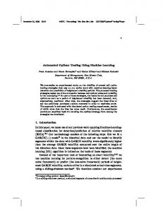
The results, however, showed that a logistic regression model could not be applied well to this set of highdimensional features. Intuitively this behavior can be explained if we consider the significant noise introduced by the high-dimensional features, which makes it difficult to fit weights for our model. More specifically, this behavior could be due to certain features obscuring patterns obtained by other features. In an attempt to reduce the dimensionality of our feature space, we use cross-validation to eliminate less effective features. We realized that logistic regression model on stock-data can fit at most two-dimensional feature space with reliability. The results of the cross validation suggested that feature(1) and feature(4) provide optimal results. In addition to optimizing the feature set, we also use cross-validation to obtain an optimal training set, which is defined as the training duration in our application. Figure 1 plots the variation of the metrics over training durations from 30-minute period to 120-minute period (the heuristic assumption is training begins at 9:30 AM, and testing 3 Our

implementation utilizes the MNRFIT library in Matlab. will denote features using ⇣ the numbering of⌘equations for the rest (t) (t 1) (t 1) of this report, e.g. feature (1) is Popen Popen /Popen ) 4 We

lasts for 30 minutes right after training finishes). We observe that logistic regression model achieves maximal performance when training duration is set to 60 minutes. Figure 1: Performance over different training durations

Hence, we train the logistic regression model with feature (1) and feature (4), starting from 9:30 AM to 10:30 AM, and the obtained model obtains precision 55.07%, recall 30.05%, accuracy 38.39%, and profit 0.0123 when testing for the rest of the day. 3.1.2

Improvements based on Time Locality

While logistic regression was able to achieve a reasonable performance with the two-dimensional feature set including (1) and (4) and made a profit of 0.0123 , we attempted to further improve our results. Based on earlier discussion, our logistic regression model is constrained to a low-dimensional feature space. As a result, we must either select more descriptive features in low-dimensional feature space or use a different model that would learn from a higher-dimensional feature space for our application.

new features based on the -minute high-low model[1]5 . Professionals in the algorithmic trading field recommended the heuristic choice of = 5.6 The -minute high-low model tracks the high price, low price, high volume, low volume across all the ticks in any -minute span. For the most recent -minute span w.r.t. any 1-minute bucket of (t) (t) (t) (t) time t, we define P H , P L , V H , V L as follows: PH

(t)

PL

(t)

VH

(t)

VL

(t)

= = = =

t t t t

max

Phigh

(i)

(7)

min

Plow

(i)

(8)

max

Phigh

(i)

(9)

min

Plow

(i)

(10)

it 1 it 1 it 1 it 1

Under the -minute high-low model, we choose our features to be the following: ⇣ ⌘ (t) (t 1) Popen Popen (11) (t) (t) PH PL ⇣ ⌘ (t) (t 1) Vopen Vopen (12) (t) (t) VH VL Specifically, they are the ratio of open price and open volume change to the most recent “ -minute high-low spread”, respectively. Considering that our stock universe may be different, we use cross-validation to determine the optimal value of . Figure 2 suggests that = 5 leads to maximal precision while = 10 guarantees maximal profit and recall. For the purpose of this project, we chose = 5 because higher precision leads to a more conservative strategy. Figure 2: Performance over different

We started by constructing more descriptive features. We hypothesized that the stock-market exhibits significant time-locality of price-trends based on the fact that it is often influenced by group decision making and other time-bound events that occur in the marketplace. The signals of these events are usually visible over a time-frame longer than a minute since in the very-short term, these trends are masked by the inherent volatility of the stock prices in the market. For example, if the market enters a mode of general rise with high-fluctuation at a certain time, then large 1-minute percentage changes in price or volume become less significant in comparison to the general trend. We attempted to address these concerns by formulating

5 Inspired 6 Keith

by CS 246 (2011-2012 Winter) HW4, Problem 1. Siilats, a former CS 246 TA

Also, we set training duration to 60 minutes based another cross-validation analysis with = 5. Our -minute high-low logistic regression model finally achieves precision 59.39%, recall 27.43%, accuracy 41.58% and profit 0.0186. Table 1: Comparison between two logistic regression models Model Baseline -HL

Profit 0.0123 0.0186

Precision 55.07% 59.39%

Recall 30.05% 27.43%

Accuracy 38.39% 41.58%

By compare the performance of the two logistic regression models in Table 1, we clearly see that -minute highlow model provides a superior model than baseline model. This result validates our hypothesis on the time-locality characteristic of stock data and suggests that time-locality lasts around 5 minutes.

3.2. Support Vector Machine As we discussed earlier, further improvement of results may still be possible by exploring a new machine learning model. The previous model we explored contained us to a low-dimensional feature space, and to overcome this constraint, we attempted to experiment with SVM using `-1 regularization with C = 1. 3.2.1

Feature & Parameter Selection

We tried different combinations of the 8 features defined by equation (1) to (6), equation (11), and equation(12). Since there are a large number of feature combinations to consider, we used forward-search to continuously add features to our existing feature set and choose the best set based on our 4 metrics. Table 2: Performance over different feature sets Features (1), (4) (11), (12) (1), (4), (11), (12) (1), (4), (11), (12), (2), (5) (1), (4), (11), (12), (2), (5), (3), (6)

Profit 0.3066 0.3706 0.3029

Precision 44.72% 42.81% 42.48%

Recall 52.11% 57.64% 47.54%

Accuracy 42.85% 40.34% 39.42%

0.3627

45.22%

56.25%

42.60%

0.3484

46.43%

55.66%

42.91%

We chose the last feature set since it leads to the highest precision and also very high profit, recall, and accuracy. In addition, we set training duration to 60 minutes using

cross-validation. Similarly, we choose optimal = 10 and C = 0.1 using cross-validation. We also compared linear kernel with Gaussian kernel, and linear kernel tends to give better results. The SVM model trained with the chosen training duration, and C finally achieves precision 47.13%, recall 53.96%, accuracy 42.30% and profit 0.3066. By comparing -minute high-low regression model with SVM model, we see that SVM model significantly improves recall, by almost 100%, by only sacrificing a small percentage of precision, around 20%. 3.2.2

Time-Locality Revisited

Recall that the -min high-low model is based on our hypothesis that there exists a minute rolling correlation in between trades within a certain period of time, and by cross-validation, we choose = 10 for the SVM model. To further substantiate this hypothesis, we conducted an experiment in which we train an SVM using the optimal parameters from the previous section, and then we evaluate the accuracy of the model by testing it on different periods of time. Specifically, the performance statistics of an SVM model, trained from 9:30 AM to 10:30 AM, are listed in Table 3. A close inspection shows that there exists a downtrend in performance as delay between testing period and training period becomes larger. In fact, it wouldn’t be surprising to see even better performance of this model within 10 minutes after training completes as we chose = 107 ! Table 3: Performance over periods of time Period 10:30-11:00 AM 10:45-11:15 AM 11:00-11:30 AM 11:15-11:45 AM 11:30-12:00 AM

Profit 0.0926

Precision 56.45%

Recall 38.10%

Accuracy 43.92%

0.0684

42.49%

38.32%

42.15%

0.0775

54.29%

41.09%

43.07%

0.0726

48.68%

36.68%

38.68%

0.0632

32.74%

29.77%

40.44%

4. Conclusion and Furtherwork Predicting stock market trends using machine learning algorithms is a challenging task due to the trends being 7 The result is precision: 68.84%, recall: 36.88%, accuracy: 44.84%, which tops all other results in Table 3.

masked by various factors such as noise and volatility. In addition, the market operates in various local-modes that change from time to time making it necessary to capture those changes in order to be profitable while trading. Although our algorithms and models were simplified, we were able to meet our expectation of reaching modest profitability. As per our sequential analysis it became clear that factoring in time-locality and capturing the features after smoothing, to reduce volatility improves profitability and precision substantially. Factoring in features of high-dimensionality after careful selection can also be significant to improving the results and our analysis of the SVM compared to logistic regression was able to capture this. We expect that this is the case because of higher-dimensionality increasing the likelihood of linear separation of the dataset. Finally, iterative improvements achieved through sequential optimizations in the form of discretization, realization of time-locality, smoothing improved results significantly. Cross-validation and forward search were also powerful tools in making the algorithm perform better. In conclusion, our experience in this project suggests that machine learning has great potential in this field and we hope to continue working on this project further to explore more nuances in improving performance via better algorithms as well as optimizations. A few interesting questions that we think would be worth investigating would be exploring other international stock markets to find locations where algorithmic trading is able to perform better. In addition, it would be interesting to investigate other algorithms such as reinforcement-learning to compare with the models discussed in this report. Feature selection has been key and more work in discovering more descriptive features would prove to be promising in terms of making the results even better.

5. Acknowledgements We would like to thank Professor Andrew Ng and the TA’s of the class for their feedback and input on the project. We would also like to thank Keith Sillats for generous help in the form of advice as well as valuable personal experience in the field that helped inform our decisions.

References [1] Jure Leskovec, TA: Keith Sillats HW 4

A. Appendix Stock Ticker APOL CBG US Equity CMA CMS CVS GCI GME GT JBL KIM LNC NFX NI NWL NYX PWR QEP SEE TER THC TIE TXT ZION

Origin US Equity US Equity US Equity US Equity US Equity US Equity US Equity US Equity US Equity US Equity US Equity US Equity US Equity US Equity US Equity US Equity US Equity US Equity US Equity US Equity US Equity US Equity