Geoscientific Model Development
Open Access
Hydrology and Earth System Sciences
Open Access
Geosci. Model Dev., 6, 1261–1273, 2013 www.geosci-model-dev.net/6/1261/2013/ doi:10.5194/gmd-6-1261-2013 © Author(s) 2013. CC Attribution 3.0 License.
ess
Data Systems
Ocean Science
Open Access
Solid Earth
Open Access
Automated tracking of shallow cumulus clouds in large domain, long duration large eddy simulations T. Heus1 and A. Seifert2 1 Max
Planck Institute for Meteorology, Hamburg, Germany Centre for Weather Research, Deutscher Wetterdienst, Hamburg, Germany
2 Hans-Ertel
Correspondence to: T. Heus (
[email protected]) Received: 26 February 2013 – Published in Geosci. Model Dev. Discuss.: 2 April 2013 Revised: 24 June 2013 – Accepted: 5 July 2013 – Published: 22 August 2013
1
Introduction
Clouds and convection are a prime example of how the many scales of atmospheric flow can interact. The typical sizes range from less than 100 m to tens of kilometers. This range is extended when one takes mesoscale organization and clustering of cloud fields into account. On the other hand, the clouds themselves are part of a turbulent field with scales going down to the millimeter range. One manifestation of this multiscale physics is the fact that the cloud size distri-
Open Access
Abstract. This paper presents a method for feature tracking of fields of shallow cumulus convection in large eddy simulations (LES) by connecting the projected cloud cover in space and time, and by accounting for splitting and merging of cloud objects. Existing methods tend to be either imprecise or, when using the full three-dimensional (3-D) spatial field, prohibitively expensive for large data sets. Compared to those 3-D methods, the current method reduces the memory footprint by up to a factor 100, while retaining most of the precision by correcting for splitting and merging events between different clouds. The precision of the algorithm is further enhanced by taking the vertical extent of the cloud into account. Furthermore, rain and subcloud thermals are also tracked, and links between clouds, their rain, and their subcloud thermals are made. The method compares well with results from the literature. Resolution and domain dependencies are also discussed. For the current simulations, the cloud size distribution converges for clouds larger than an effective resolution of 6 times the horizontal grid spacing, and smaller than about 20 % of the horizontal domain size.
bution has frequently been reported as something similar to Thewith Cryosphere a power law distribution, an exponent close to 2, depending on the type of cloud field studied. This means not only that clouds show some self similarity leading to a scalefree distribution, in fact a value of 2 for the slope of the power law distribution would mean that all cloud sizes in this scale range have a similar contribution to the total cloud cover (e.g., Wood and Field, 2011; Zhao and Di Girolamo, 2007). It stands to reason that other cloud properties such as entrainment, cloud depth or cloud lifetime also show a dependency on cloud size (e.g., Dawe and Austin, 2013). Last but not least, it seems obvious and has been confirmed by observations (e.g., Byers and Hall, 1955) that rain formation depends on cloud size (and other related properties like cloud depth). Although such a dependency might be obvious from the phenomenology of clouds, it is difficult to quantify because the details of the cloud life cycle of such shallow and rather short-lived clouds are very difficult to observe in the field. An attempt to approach the problem from a more theoretical point of view has been made by Seifert and Stevens (2010), who use the concept of a Damk¨ohler number, a dimensionless number that is the ratio of cloud lifetime and a microphysical timescale. While the cloud lifetime characterizes the dynamics of the cloud, the microphysical timescale quantifies the time needed to form rain. Only clouds with a Damk¨ohler number larger than one would form rain, i.e., when the microphysical timescale is smaller than the cloud lifetime. This shows that studying the cloud size distributions and the cloud life cycles of individual clouds may be key to gain a deeper understanding of, for example, cloud cover and rain formation. Not only the rain formation, but also the cloud transport shows a non-trivial dependency on the cloud
Published by Copernicus Publications on behalf of the European Geosciences Union.
M
1262 life cycle: as reported by Heus et al. (2009), a typical cloud life cycle can be built from several distinct pulses that follow one another in time. Knowing the cloud size distribution may also help to develop parameterizations of clouds and convection which are scale adaptive. Similar to the Smagorinsky closure in large eddy simulations (LES) models, which make use of the selfsimilar power law spectrum in the inertial subrange of turbulence for the closure, one could make use of the cloud size distribution to construct cloud schemes that parameterize only the unresolved scales smaller than a given grid size. This is especially important, since the horizontal resolutions of numerical weather predictions (NWP) models approach grid sizes for which the assumptions of the classical convection schemes (e.g., Tiedtke, 1989; Neggers et al., 2009) do no longer hold, i.e., a scale separation between the largescale resolved flow and the convective regime does no longer exist in these models. It then becomes necessary to take a scale-aware approach to the convection parameterization, where the cloud field is partially resolved, while the smaller scales still need to be accounted for in a sub-grid model. This is also the regime where spectral cloud schemes, in the tradition of Arakawa and Schubert (1974), will see part of their cloud spectrum being resolved, while other clouds are not. In other words, the properties of individual clouds become relevant for the parameterization as the statistical convergence of the mean properties of the field begins to break down. One approach to design a parameterization that works on coarse and on fine grids alike, is to describe the cloud properties (e.g., thermodynamic quantities, entrainment and detrainment rates, and mass fluxes) as a function of the cloud size distribution. Potentially, the cloud properties also depend on the life cycle of the cloud, that is, whether the cloud is young and emerging, mature, or in the decaying phase of its life. Plant and Craig (2008) took the first steps to such an approach for deep convection, but nothing has been done for boundary layer clouds yet. To develop scale-aware shallow convection schemes based on the results of fine-scale LES (1x ≈ 25 m), it is necessary to be able to track shallow clouds in time and space. Although such tracking has been done before (e.g., Zhao and Austin, 2005; Plant, 2009; Heus et al., 2009; Dawe and Austin, 2012), many of these studies report issues that make it challenging to perform cloud tracking efficiently for a setup that fits our current requirements. For instance, we require the following. 1. To study simulations with a sufficiently long duration, at least much larger than the maximum lifetime of any cloud in the system (over 24 h). 2. High enough resolution to accurately capture the smallest clouds in the system (down to 25 m horizontal resolution).
Geosci. Model Dev., 6, 1261–1273, 2013
T. Heus and A. Seifert: Tracking of shallow cumulus clouds 3. Large enough domains to ensure a statistical convergence for all cloud sizes, and to be able to mimic the horizontal grid size of a climate model (around 50 km). 4. To include the tracking of rain and subcloud thermals to be able to study the full cycle of processes. The approach for cloud tracking presented in the current paper attempts to solve these issues. The algorithm combines methods presented by previous authors, but optimized such that it is feasible for relatively long simulations of large fields of cumulus clouds, including fields with very many small clouds (about 100 m wide) or fields that include more organization and some hints of deepening and massive cloud top detrainment, where the convective elements can be in the range of a few kilometers, with outflow regions in the same range. Tracking of clouds has been done before. Radar observations with suitably high temporal and spatial resolutions allow for tracking (e.g., Handwerker, 2002) and life cycle studies of individual cumulus clouds. These algorithms tend to focus on overcoming issues that are specific for radar, such as attenuation and limited amount of measured properties, and on pattern recognition after advection of the cloud field with the mean wind. For cloud tracking in LES, no correction is necessary for attenuation, and all properties of the cloud are available for every neighboring grid cell. Also, the difference in the cloud fields between two subsequent time steps is usually small enough, so that it is not necessary to develop a complicated pattern recognition and advection algorithm. Direct connectivity suffices. This is typically done by grouping all grid cells with a finite liquid water content that are next to each other in three-dimensional space and in time as a single cloud. This lies at the core of many previous tracking algorithms (Zhao and Austin, 2005; Heus et al., 2009; Plant, 2009; Dawe and Austin, 2012). Two particular issues arise when using this four-dimensional connectivity in its purest form: (1) the amount of data becomes prohibitive for larger domains or longer time series; and (2) it turns out that many clouds that are clearly separated processes for all purposes are connected to each other by a brief connection of the two at some point in time, and the algorithm would then categorize all these clouds as one single system. This obviously defeats the purpose of tracking individual clouds. To overcome the problem of overly connected cloud systems, several methods have been developed. For example, Zhao and Austin (2005) and Heus et al. (2009) used a visual inspection to select clouds from LES. This labor-intensive method allowed for the selection of up to 35 clouds per simulation for closer inspection. Dawe and Austin (2012, hereafter DA12) used a combination of liquid water content (“the cloud”) and buoyancy (“the cloud core”) for their cloud tracking, and were able to automate the cloud selection. In this way, they were able to track up to 2381 clouds; enough www.geosci-model-dev.net/6/1261/2013/
T. Heus and A. Seifert: Tracking of shallow cumulus clouds to see statistical convergence of the first order statistics, at least for the (more numerous) smaller clouds. Plant (2009) overcame the issue of overly connected systems by only considering time in the forward direction, without going back in time. This approach has the additional advantage that it becomes more feasible to perform the cloud tracking online, during the LES run, reducing the I/O (input/output) footprint and the post-processing time. However, this one-way connectivity is problematic in the cloud initiation stage, where a subcloud thermal reaches lifted condensation level (LCL) at several locations at once to create several small cloudy areas that later merge into a single coherent cloud. A forward-in-time tracking scheme would register those clouds as separate, instead of part of a single coherent system. While this may be a valid simplification for deep convective clouds, it is a potential issue for a field of many, short lived, shallow cumulus clouds. All of the approaches mentioned in the previous paragraph perform their cloud tracking in time and in three spatial dimensions, making the tracking expensive for larger data sets. To mitigate the computational cost, Jiang et al. (2006), reduced the dimensionality of the problem by tracking the projected cloud cover instead of the 3-D cloud field. Although this simplifies the problem tremendously from a computational point of view, it also increases the risk of merging of separate convective pulses. In this paper, we attempt to combine the sophistication of DA12 with the economy of Jiang et al. (2006) by tracking the projected cloud cover, while taking the local cloud top and cloud base into consideration. The developed algorithm also takes splitting and merging events into account, and we track the subcloud thermal (as was done by DA12) and the areas of precipitation. As Heus et al. (2009) and DA12 argued, various clouds tend to connect briefly in time. A method purely based on connectivity would count those clouds as a single cloud. However, many properties of the clouds, including the cloud life cycle, the scalar transport and the precipitation, are more likely a function of the cloud size of the single convective entities than of the entire merged set of clouds. Therefore, it is necessary to split those extended regions of liquid water into separate clouds. For this, a splitting algorithm is presented, based on dividing the cloudy areas between the separate convective cores. An additional advantage of such a splitting algorithm in our 2-D tracking scheme, is that it helps the algorithm to distinguish large outflow regions from small convective cores underneath. Still, it should be emphasized that the algorithm is not designed for multilayer systems. As a natural result of the splitting of clouds with our algorithm, the clouds can be categorized based on whether or not they host a buoyant core, or whether or not they actually have been subject to the splitting algorithm. Depending on these categories, the cloud properties may differ significantly. Not every category may be of relevance for every study. For instance, passive clouds are usually not expected to contribute www.geosci-model-dev.net/6/1261/2013/
1263 much to convective transport, but they may very well contribute to the cloud cover. In this model development paper, we will discuss the methodology of the tracking algorithm and compare our results with previous studies. Subsequent studies on the physics of the cloudy atmosphere will follow in later papers. This paper starts with a brief description of the LES case that we use for validation of the tracking algorithm in Sect. 2. After that, we describe the tracking itself in Sect. 3. A first visual inspection is presented in Sect. 4, and Sect. 5 compares our current results with older work, such as DA12 and Neggers et al. (2003), with a focus on cloud size distributions and probability density functions. The categorization into passive and active clouds allows for some sanity checks of the tracking algorithm, which we will also discuss in Sect. 5. 2
LES case description
We base the evaluation of the feature tracking module on a LES run of shallow cumulus clouds, following the case setup of the Rain In Cumulus over the Ocean (RICO) intercomparison study (vanZanten et al., 2011). This regime features some intermittent precipitation that often evaporates before it hits the surface. When the cloud layer develops, cloud tops reach up to 3 km, and some anvil-like outflow occurs. In the standard RICO simulations, the lifetime of these outflow regions is limited, resulting in little overlap with new clouds at lower levels. The simulation is performed using the UCLA LES model (Stevens et al., 2005; Savic-Jovcic and Stevens, 2008) with a duration of 40 h. By default, the scalar advection is done using a slope limited monotone advection scheme (van Leer, 1979). When testing the sensitivity to the resolution and advection scheme in Sect. 5.3, a second-order upwind scheme is used. The output time step 1t requires some consideration; a very small time step quickly results in an unmanageable amount of data, but the time step needs to be sufficiently small so that clouds do not advect so fast through the grid that the connection in time is missed. In other words, a Courantlike criterion needs to be fulfilled: Co =
U 1t < 1, 1x
(1)
where U is the horizontal velocity of the structures, and 1x the horizontal grid size. Note that U is the velocity with respect to the computational grid. In the current run, a Galilean transformation has been applied on the simulation that subtracts the mean wind from the flow. This leaves only the (small) deviations with height from this mean wind to be considered in the Courant number. For these simulations, 1t = 60 s was sufficient. A minor advantage of the tracking in 2-D is that the velocity of the projection of structures is lower than the velocity in the 3-D field, which relaxes the Courant criterion a bit.
Geosci. Model Dev., 6, 1261–1273, 2013
1264
T. Heus and A. Seifert: Tracking of shallow cumulus clouds
Since the smallest clouds tend to dominate the cloud size distribution (CSD), we use a relatively fine resolution of 1x = 1y = 1z = 25 m. To alleviate the limitation of cloud size by the size of the computational domain, we use a horizontal domain size of 25 km × 25 km. The first 4 h of the simulation are discarded as spin up. 3 3.1
Tracking methodology General overview
Our methodology consists of tracking projected areas of cloud, cloud core, rain and subcloud thermals in time and space, by simply connecting adjacent points in space and time that fulfill the criteria for being a cloud, core, rain or thermal. To perform the full tracking, 10 LES output fields are necessary (all as a function of (x, y, t)). For clouds: the liquid water path (LWP), cloud core, cloud base and cloud top. For rain: the rain water path (RWP), the rain base and the rain top. For thermals: the thermal scalar path, base and top (see Sect. 3.2). A flowchart with a pseudo code description of the algorithm is shown in Fig. 1. Every cloud consists of all the connecting columns with a cloud LWP (x, y, t) over a threshold of 5 g m−2 . In addition, the cloud base of each column needs to be below the cloud top of the other column. That is, if a certain point (x, y, t) has sufficient liquid water path, the algorithm will check whether (x ± 1x, y, t) fulfills the criteria as well, and the cloud base of either cell is not higher than the cloud top of the other column, which would suggest multiple cloud layers. This procedure is then followed in the other direction for (x, y ± 1y, t), and also in time for (x, y, t ± 1t). This procedure is performed recursively, until all the connecting cloud columns are discovered and none of the neighboring columns have a sufficient liquid water path and matching cloud extent. Rain areas are tracked using the neighboring columns with a RWP(x, y, t) over a threshold of 5 g m−2 . Subcloud thermals are tracked using a designated scalar, as described in Sect. 3.2. As for clouds, neighboring rain or thermal points are required to have a matching vertical position. Cloud cores are mainly used for the cloud splitting algorithm, which is described in Sect. 3.3. Finally, thermals, clouds, and rain patches are connected to each other if they share at least one grid cell (in x, y, z, t) with each other in a parent/child relationship. That is, a thermal that connects with a cloud can be seen as the parent of that cloud, and a cloud that connects with a rain patch can be seen as the parent of that rain patch. That way, surface precipitation can be traced back to the cloud that generated it, or clouds can be traced back to their subcloud thermals.
Geosci. Model Dev., 6, 1261–1273, 2013
3.2
Thermal tracking
To track the subcloud layer thermal, we use an additional prognostic scalar as introduced by Couvreux et al. (2010) and also used by DA12. This scalar C(x, y, z, t) is emitted from the surface, and then decays over time with a timescale τ0 : C(x, y, z, t) dC(x, y, z, t) =− , (2) dt τ0 decay with τ0 = 1800 s sufficiently close to the typical timescale of the boundary layer, and a constant scalar surface flux as its boundary condition. Since the scalar has no real physical meaning, the actual value of the scalar (and of its surface flux) is irrelevant. A high scalar concentration means that a parcel of air has been in contact with the surface relatively recently. This allows us to define a thermal without making any assumptions on the properties of the thermal, such as its velocity or buoyancy. To use this scalar for thermal tracking, we need to define when the scalar concentration is high enough in a way that works for every level in the convective boundary layer. Following Couvreux et al. (2010), we define a grid cell (x, y, z, t) to be in a thermal T if its scalar value is at least 1 standard deviation σC (z, t) over the slab average: (x, y, z, t) ∈ T if
C((x, y, z, t)) − C(z, t) > 1. σC (z, t)
(3)
To get a column representation of the thermal field, the sum of this normalized scalar excess over σC (z, t) is recorded, including the lowest and highest location that fulfills this criterion. The tracking is then done in a similar way as the tracking of the clouds and thermals. To eliminate pollution by areas with a scalar value around the threshold, we require thermals to have a point in the lower half of the subcloud layer at some point in their lifetime, and to be at least four-cells large in space and/or time. 3.3
Cloud splitting
A common issue in cloud tracking (see e.g., DA12 and Heus et al., 2009) is that cloudy objects tend to interact with other clouds, while largely keeping their own properties. Connecting these clouds into one large cloud system would negate the point of doing life cycle studies. These collisions are more likely to happen in 2-D tracking than in 3-D tracking, since overlapping, non-touching, cloud layers would be counted as a collision. Therefore, a cloud splitting algorithm is necessary. Our algorithm is conceptually similar to the one presented by DA12, but different in implementation because of the 2-D tracking. We start with tracking not only the clouds, but also the cloud cores, defined as columns where the maximum incloud θv excess is over some threshold, chosen to be 0.5 K. To eliminate noise around this threshold, we also require that www.geosci-model-dev.net/6/1261/2013/
T. Heus and A. Seifert: Tracking of shallow cumulus clouds
Start
Thermals Track
Cores Track
1265
Clouds Track Split around cores Connect with thermals
Rain Track Connect with clouds
Output
Split(parentcells,childcells) connect(parentcells, childcells) loop(n1=1,nr childcells) if(nr parents(n1) == 0) childcell(n1) is passive elseif(nr parents(n1) == 1) childcell(n1) is single plume else for all regions(parentcell/=NaN) region is new active cell regiongrowing(childcell(n1),activecells(:,n1)) for all unclaimed regions region is new remnant all regions are siblings
Track(cell) loop (x,y,t) if (newcell(x,y,t) == true) nelement = 0 growcell
Growcell(x,y,t) nelement = nelement + 1 cell(nelement)(x,y,t) = (x,y,t) if (newcell(x+1,y,t) == true) growcell if (newcell(x--1,y,t) == true) growcell if (newcell(x,y+1,t) == true) growcell if (newcell(x,y--1,t) == true) Connect(parentcells,childcells) loop(n1=1,nr parentcells) growcell loop(n2=1,nr childcells) if (newcell(x,y,t+1) == true) if (any(parentcell(n1,x,y,t)==childcell(n2,x,y,t))) growcell parentcell(n1) is parent of childcell(n2) if (newcell(x,y,t--1) == true) childcell(n2) is child of parentcell(n1) growcell
Regiongrowing(childcell,activecells) loop (niter=1,maxiter) loop (n=1,nr parentcells) where (activecell(n, x, y, t) is next to any(childcell) if(location unclaimed by other parents) add location to activecell(n)
Fig. 1. Flowchart of the tracking algorithm in pseudo code. Tracking is first performed for thermal, then for cloud cores, clouds, and rain using a recursive cell growing method. Additionally, clouds are being split into multiple cells when appropriate, and are connected to thermals and rain areas, respectively, that share the same location at some point in the lifetime of the cells. The splitting algorithm makes use of the connecting algorithm and of the region growth algorithm that is slightly different from the cell growth used for the tracking.
the core regions have at least one cell in the lower half of the cloud layer, and that they are at least four-cells large (in space and/or time). Clouds that contain no cores are passive clouds and do not need any splitting. Clouds that contain exactly one core are called active clouds, but since they are isolated pulses that are not part of a bigger system of multiple pulses, they do not need any splitting either. If a cloud (system) contains more than one core, we follow the splitting algorithm as schematically depicted in Fig. 2 for a system with two cores, the dark red and green areas in Fig. 2a. This is performed by the region growing subroutine in Fig. 1. We allow these cores to grow incrementally into the surrounding cloud area that has not yet been taken by another core (Fig. 2b). This region growth happens in space as well as time. Since the larger cores (such as the red core in Fig. 2) have a larger circumference, they have more points participating in this region growth, and are therefore expected to pick up a larger part of the cloud. Since these cores grow through the time dimension as well as through space, the largest cores are expected to capture points that lie relatively far away from their center. To limit the effects of fresh cores growing under an outflow remnant of an older cloud, region growth is only allowed if the vertical distance between the cloud base of the two columns is less than 300 m. The number of iterations is limited proporwww.geosci-model-dev.net/6/1261/2013/
tionally to the area of the original core, although the results show little sensitivity to this parameter. The region’s growth continues until no core has any iterations left, or until all possible growing paths are covered (Fig. 2c). Finally, the parts of the cloud that has not been covered, is either allocated to its neighboring core if there is only one connecting core, or is left as a separate remnant cloud if multiple cores are connected to the region (Fig. 2d). The regions that are allocated to a specific core are now pulses within a multipulse system. 3.4
Performance
Although tracking can in principle be done online, during the actual LES simulation, the spatial parallelization of the code and the requirement that the entire lifetime of each cloud needs to be considered simultaneously yields practical implementation issues and concerns with the load balancing of the simulation. Therefore, the cloud tracking is applied offline, as a post processing step. Although our required data set is not as big as for DA12, a large data set can pose some storage and I/O issues. As an illustration, the biggest simulations that we performed the cloud tracking on thus far had 2048 grid cells in each of the horizontal directions, and 2400 time steps (40 h), resulting in 400 GB of data necessary for the tracking, not counting additional scalars of interest such as Geosci. Model Dev., 6, 1261–1273, 2013
1266
T. Heus and A. Seifert: Tracking of shallow cumulus clouds a)
b)
c)
writing out the data to and from the hard drive. Obviously the 3-D tracking is a very different and potentially more precise approach, but this processing time compares well with the 1 h 40 min reported by DA12 for 3 h of BOMEX (Barbados Oceanographic and Meteorological Experiment) clouds with 256 cells in the horizontal directions. In some sense, the strain that is being put on the system by the cloud tracking is good news: all components, including storage and memory, but also I/O bandwidth and CPU power during the simulation as well network bandwidth to download the data from the supercomputer, are close to their limitations, meaning that there is no individual bottleneck in the present system. However, in the near future, performing simulations on larger domains is more feasible than doing the tracking on those simulations. In those cases, some spatial averaging of the input data is likely necessary. Given that the effective resolution of LES simulations is always coarser than the grid resolution (see also Sect. 5.3), these kinds of optimizations should be feasible.
4
d)
Fig. 2. Schematic representation of cloud splitting. A cloud (a; the blue area, solid line) with multiple distinct cores (the red and green areas in a, dashed lines) is divided between the two cores by use of the region growing process, the lighter red and green regions in (b) and (c). Sudden increases in local cloud base are avoided. The remaining cloud, the blue parts in (c), are assigned to their respective cores if no other core connects to these areas, or are treated as separate remnants if multiple cores are connected to them, the blue area in (d). Actual splitting occurs in three dimensions (x, y, and t) instead the two depicted. The figure displays the cloud splitting in two dimensions out of x, y, and t; the algorithm works similarly in the third dimension. For further details, see the text.
surface precipitation or in-cloud velocity, humidity and temperature. Furthermore, much of the data has to be stored in memory during the tracking. To mitigate this memory limitation, we internally use 2-byte integers for our cloud tracking, reducing the memory footprint by almost 50 %. Still, the cloud tracking has a peak memory usage of up to 200 GB for the biggest runs, and these amounts of shared memory are not very common. As long as the data can be contained in the physical memory of the computer, the tracking itself takes less than 1 h, most of which is spent reading in and Geosci. Model Dev., 6, 1261–1273, 2013
Visual inspection
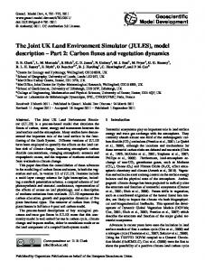
Before discussing the actual results of the tracking, it is worthwhile to explore whether the 2-D approximation is valid for these cloud fields. Therefore, it makes sense to briefly study the vertical structure of the cloud field first. Figures 3, 4, and 5 show snapshots of the feature tracking during simulation. These figures are part of animations that are available as supplementary material to this paper. In Fig. 3, a vertical cross section of the humidity fluctuations around the slab mean is shown with the thermals, clouds and rain areas in contours around it. Note that the actual tracking is performed with the projection of all these fields. As can be inferred from Fig. 3 and its related animation, multiple cloud layers (or thermals, rain) are rare, so recording the top and base point of each object in every column should give an accurate description of the object’s geometry. In Fig. 3 it can also be seen that thermals and clouds tend to be well connected – although not always and not consistently. The thermals are also relatively narrow, and seemingly short lived. Part of this is deceptive because the mean wind perpendicular to the cross section of around –3.5 m s−1 transports the features through the cross section. Part of this is also due to the choice of criteria for the thermal air, which is more focused on capturing the part of the thermal that is truly doing the upward transport and ignoring some broader parts beyond the buoyant core of the thermal. Figure 4 shows the clouds at t = 24 h after processing the data through the tracking and splitting algorithm. Areas with the same color are part of the same cloud, meaning that areas with the same color that are currently separated from each other were once, or will be later, connected in space. On the other hand, currently connected areas with different colors are apparently part of different pulses and harbor separate www.geosci-model-dev.net/6/1261/2013/
z (km)
T. Heus and A. Seifert: Tracking of shallow cumulus clouds
1267
3 2 1 12 2
0 x (km) 0 qt excess [gkg-1 ]
12 2
Fig. 3. xz cross section of the simulation at t = 24 h. Background color field represents deviations from the mean total specific humidity qt . Red contours depict the thermals, blue contours the clouds, black contours rain patches.
Cloud Number t = 24.02 h 10
y (km)
5 0 5 10 10
5
0 x (km)
5
10
Fig. 4. Projection of the cloud field at t = 24 h. Every patch of the same color depicts a single cloud after the application of the splitting algorithm. Colors are assigned randomly; very similar colors may be used occasionally for different clouds.
cores at some point during their life. The splitting algorithm seems to behave well and the size of the structures is in line with expectations. However, the region growing methodology imposes a shape on some of the clouds, especially on the division between active pulses and small remnants. Later in the simulations, massive outflow regions are usually recognized, but some artificial cloud shapes can be seen as well. This may limit the reliability of the method for certain applications. In Fig. 5 the same snapshot is shown as in Fig. 4, but now with the colors depicting the type of the cloud after application of the splitting algorithm: magenta clouds are pas-
www.geosci-model-dev.net/6/1261/2013/
sive, black clouds are single pulse clouds, and blue clouds are remnants of the red, active multipulse clouds. From this figure and from the accompanying movie it can be seen that the active clouds are at least visually dominant. Remnants of clouds often appear late in the life cycle of a cloud system, on the down shear side of the active clouds, and are often part of the outflow regions of the larger clouds, with low liquid water path and high cloud bases. Overall, a variety of cloud sizes can be observed, with instantaneous cloud fields emphasizing the tail ends of the distribution, while the connectivity in time and the splitting of cloud systems emphasizes the mid-sized clouds.
Geosci. Model Dev., 6, 1261–1273, 2013
1268
T. Heus and A. Seifert: Tracking of shallow cumulus clouds
Cloud Type t = 24.02 h
Table 1. Number and average fractional cover of thermals, clouds and rain patches in 40 h of RICO simulations.
10 Thermals Clouds – of which passive – of which single pulse – of which remnant – of which part of multipulse – without splitting Rain
y (km)
5 0 5
Frac. Cover
424 992 1 061 188 555 791 2124 486 112 17 161 559 342 7557
3.7 % 13.8 % 1.02 % 0.55 % 3.45 % 8.81 % 13.8 % 3.5 %
Size Distribution
10-6
10
Number
Cloud Thermal Rain
10
5
0 x (km)
5
10
Fig. 5. The same projection of the cloud field as Fig. 4, but with the color depicting the type of cloud: magenta clouds are passive, black clouds are single pulse clouds, and blue clouds are remnants of the red active multicell clouds.
Frequency of occurence (m-3 )
10-7 10-8 10-9 10-10 10-11
5 5.1
Validation
10-12
Distributions of thermals, clouds and rain
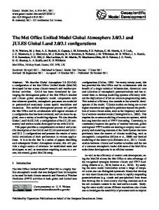
The first quantitative results from the tracking are the total number and area of the objects (Table 1), and the size distributions of the thermals, clouds and rain objects in Fig. 6. In Table 1, it is clear that the number of clouds is overwhelmingly dominated by the passive clouds and the remnants, both of which are non-buoyant. The cloud cover, however, is dominated by the convective pulses. The cloud size distribution shows the characteristic power law behavior, with a scale break around a cloud size of around 1 km. The thermal cover is relatively small, a sign of both the weak subcloud convection in marine boundary layers, and perhaps also of the strict definition of thermal air, being at least 1 σC over the slab mean value for the thermal scalar. However, the thermal size distribution does show a power law behavior, with a scale break close to the size of the subcloud layer depth of 500 m. In Table 1 it is clear that the number of precipitation events is relatively small, which is to be expected for shallow cumulus clouds, while the area covered by precipitation is relatively large.This is in agreement with the general notion that in a field of trade wind cumuli, only the largest clouds precipitate. This notion is further emphasized in the relatively flat rain patch size distribution in Fig. 6. The cloud size distribution in Fig. 6 is similar to the thermal size distribution for the smallest clouds. On the other Geosci. Model Dev., 6, 1261–1273, 2013
102
103 Cloud Size (m)
104
Fig. 6. Size distribution averaged over the entire simulation for clouds, thermals and rain.
hand the largest clouds have sizes similar to the largest rain patches. This in agreement with the notion of subcloud thermals being the production mechanism for the clouds, and rain being at least one of the destructive mechanisms. One could argue that no rain patch can be larger than the largest clouds, thus the maximum cloud size setting the maximum size of the rain patch. However, one could also argue the other way around, that for certain cloud sizes and lifetimes, the conversion of cloud water to precipitation becomes so efficient that this effectively limits further growth of the clouds. 5.2
Comparison with previous work
In Fig. 7, the cloud size distribution is plotted, together with best fits to a power law between 400 and 1000 m. It is not clear from the literature that a distribution of shallow cumulus clouds has to obey a power law distribution from a theoretical point of view. Many studies do however fit their cloud size distributions to a power law, and it is therefore instructive for us to do the same and compare the slope parameter with previous studies. A few things are notable when comparing these figures with those of Neggers et al. (2003) and www.geosci-model-dev.net/6/1261/2013/
T. Heus and A. Seifert: Tracking of shallow cumulus clouds
1269
Cloud Size Distribution - no tracking
10-8
10-8
10-9
10-9
Frequency of Occurence (m-3 )
Frequency of Occurence (m-3 )
Cloud Size Distribution - after tracking
10-10 10-11 10-12 10-13
8 - 16 hr, slope = -2.72 16 - 24 hr, slope = -2.69 24 - 32 hr, slope = -2.66 32 - 40 hr, slope = -2.84 102
Cloud Size (m)
10-10 10-11 10-12
103
10-13
8 - 16 hr, slope = -2.42 16 - 24 hr, slope = -2.51 24 - 32 hr, slope = -2.46 32 - 40 hr, slope = -2.61 102
Cloud Size (m)
103
Fig. 7. Cloud size distribution after tracking. Solid lines are the averages over 8 h intervals, dashed lines are the best power law fit to the data between 400 and 1000 m, with a respective slope given in the legend.
Fig. 8. Cloud size distribution without tracking. Solid lines are the averages over 8 h intervals, dashed lines are the best power law fit to the data between 400 and 1000 m, with a respective slope given in the legend.
DA12. First of all, the slope averages around –2.7, steeper than values of around –1.8 reported in the older work. Secondly, the scale breakaway from the power law fit becomes less pronounced with time. Part of this might be because RICO is slightly deeper than the BOMEX case that Neggers et al. (2003) and DA12 discussed. Deeper cloud fields tend to be more efficient in allowing mid-sized clouds to grow to sizes beyond the original scale break while leaving the number of small clouds unchanged, thus steepening the slope of the cloud size distribution in the middle of the distribution, and extending the power law behavior to larger cloud sizes. Our simulations are also run on larger domains, which are necessary to allow clouds to grow beyond the scale break size of DA12. The current results also do not show a power law behavior down to the smallest scales, in contrast with the other studies. This could be caused by the differences in horizontal resolution and scalar advection scheme. These numerical dependencies are discussed in Sect. 5.3. To be able to compare Fig. 7 to the cloud size distribution as would have been obtained following the method of Neggers et al. (2003) or Zhao and Di Girolamo (2007), Fig. 8 shows the cloud size distribution for the RICO case without applying the tracking algorithm. That is, object identification is done by performing the connectivity not in time, but only in space. Comparing Figs. 7 and 8 with each other, one can see the effects of the tracking algorithm. Similar to DA12, the tracking reduces the number of small clouds because it corrects for broken off chunks, splits up the largest clouds and emphasizes the mid-size clouds. The obtained exponent of –2.2 is in agreement with Zhao and Di Girolamo (2007), although it is significantly steeper than the –1.8 as reported by Neggers et al. (2003).
Figures 9–12 show the distributions for cloud lifetime, volume, minimum cloud base and maximum cloud top, similar to Fig. 6 in DA12. Furthermore, we have plotted the four different cloud types following the splitting algorithm as explained in Sect. 3.3. Since these figures show the histograms, the sum of the different types, represented by the colored lines, always equates the histogram for all the clouds together, represented by the thick gray line. The overall shape of the profiles is similar to the results reported by DA12, although the RICO clouds, again, tend to be longer-lived and larger. The shape of the cloud size distribution can be understood since the tracking algorithm allows us to study the different cloud types. Two regimes can be clearly distinguished: the non-buoyant remnants and passive clouds dominate the distribution on the small end of the spectrum. The large, long-lived clouds on the other hand are predominantly part of a multicore system. Within the various cloud types, the cloud lifetime follows an exponential- or gamma-like distribution. Regarding the mean volume, or mass (Fig. 10) , the passive clouds dominate the smaller side of the distribution, and the multipulse clouds dominate the larger side. Irrespective of the cloud type, the minimum cloud base distribution in Fig. 11 shows a maximum close to the lifted condensation level (LCL), simply because of the large cloud fraction around LCL. For the active clouds, few clouds have a minimum cloud base much above LCL. On the other hand, passive clouds driven by gravity waves can occur at any level in the cloud layer, and outflow remnants of larger cloud systems dominate the distribution at higher altitude, especially at levels above the cloud layer inversion. As can be expected from the cloud volume and cloud base distributions, the cloud top distribution shows a maximum
www.geosci-model-dev.net/6/1261/2013/
Geosci. Model Dev., 6, 1261–1273, 2013
1270
T. Heus and A. Seifert: Tracking of shallow cumulus clouds
Cloud Life Time
Frequency of occurence (m-3 min-1 )
10-8 10-9 10-10 10-11 10-12 0
30
60 Life time (min)
90
Fig. 9. Histogram of the cloud lifetime for all clouds, and for the different cloud types.
All Clouds Passive Single Pulse Remnant Pulse
Frequency of occurence (m-5 min-1 )
10-13 10-14 10-15 10-16 10-17
0.2
0.4 0.6 Volume (m3 )
0.8
10-11 10-12 10-13 500
1000
1500
2000 2500 Height (m)
3000
3500
4000
Maximum Cloud Top Height
10-8
10-18 10-190.0
10-10
Fig. 11. Histogram of the minimum base height for all clouds, and for the different cloud types.
Mean Cloud Volume
10-12
All Clouds Passive Single Pulse Remnant Pulse
10-9
10-14 0
120
Frequency of occurence (m-3 min-1 )
Frequency of occurence (m-2 min-2 )
10-7
Minimum Cloud Base Height
10-8
All Clouds Passive Single Pulse Remnant Pulse
10-9 10-10 10-11 10-12 10-13 10-14 0
1.0 1e8
All Clouds Passive Single Pulse Remnant Pulse
500
1000
1500
2000 2500 Height (m)
3000
3500
4000
Fig. 10. Histogram of the mean volume for all clouds, and for the different cloud types.
Fig. 12. Histogram of the maximum top height for all clouds, and for the different cloud types.
only slightly above LCL for the small passive clouds, and the remnants have a cloud top height distribution that largely coincides with its minimum cloud base height distribution, especially for the levels that can be associated with outflow from the large systems. For the highest clouds, the distribution of the remnants collapses with the distribution of the active parts of the cloud systems. These multipulse clouds show a tendency to become somewhat bigger than the single pulse clouds, and only the multipulse clouds grow deep enough to contribute to the growth of the cloud layer through entrainment of free tropospheric air. However, both single pulse and multipulse clouds show a maximum cloud top well above LCL, once again showing their buoyant, convective nature.
Overall, most of the tracking results agree well with the results of DA12, and disagreements can be explained by differences in the case setup and in the splitting algorithm. To conclude this section, we will now discuss some issues of sensitivity of our results to numerical artifacts.
Geosci. Model Dev., 6, 1261–1273, 2013
5.3
Parameter, resolution and domain size dependency
Sensitivity to the tracking parameters has been tested. Most parameters, including the details of the splitting algorithm, show little impact in the current simulations. The only parameter that does show a significant impact is the liquid water path threshold used as a basis for the connectivity of the clouds. This is not surprising, since a higher threshold will leave the smallest clouds undetected and decrease the size of the larger clouds. Furthermore, a higher threshold will www.geosci-model-dev.net/6/1261/2013/
T. Heus and A. Seifert: Tracking of shallow cumulus clouds
www.geosci-model-dev.net/6/1261/2013/
Cloud Size Distribution - after tracking
Cloud Size Density (m-3 )
10-8 10-9 10-10 10-11 10-12 10-13
LWP = 50 g kg-1 , slope = -2.23 LWP = 20 g kg-1 , slope = -2.79 LWP = 10 g kg-1 , slope = -2.89 LWP = 5 g kg-1 , slope = -2.84 LWP = 1 g kg-1 , slope = -2.56 102
Cloud Size (m)
103
Fig. 13. Cloud size distribution as a function of the liquid water path threshold for hours 32–40 of RICO. Dashed lines denote the best fit power law between 400 and 1000 m; the numbers are the respective exponents of these power laws.
Cloud Size Distribution
10-3
Large Domain No Limiter Limiter
10-4 Frequency of Occurence (m-3 )
decrease the amount of splitting and merging events between clouds. Therefore, the highest sensitivity to changes in the liquid water path threshold can be found in the cloud size distribution after tracking (Fig. 7). In Fig. 13, this cloud size distribution is plotted for several values of the liquid water path threshold. The sensitivity appears to be mostly of a quantitative nature, that is, the slope changes as a function of the threshold, but the qualitative shape of the distribution remains robust. For large thresholds, the differences in the cloud size distribution are distinct; for thresholds below 10 g kg−1 the distribution seems to converge. There is no clear cut answer to what the correct value of the threshold should be; this depends on the application. If one is more interested in studies of convection, a relatively high threshold might be useful to focus on the strongest clouds; if one is more interested in the radiative properties of clouds, a lower threshold might include more of the total cloud cover. The value of 5 g kg−1 , which is used in the current study, is sufficient for the latter goal: capturing most of the clouds, while focusing on the ones that have a significant albedo. One discrepancy between Fig. 8 and earlier results such as in DA12 and Neggers et al. (2003) is that the power law in the earlier results can be extended down to the resolution of the simulation, while the current results show fewer small clouds. One reason for this could be the use of a monotone flux-limiter scheme for the scalar advection; such schemes tend to be less dispersive than (for instance) central differencing schemes, at the cost of higher numerical diffusion. To test this hypothesis, additional runs of the first 8 h of RICO were performed, varying the horizontal resolution, domain size, and the use of the limiter. For these experiments, the default simulation had a horizontal domain size of 6.4 km and a horizontal resolution of 1x = 25 m; higher resolution simulations are performed on a 10 or 5 m resolution. The vertical resolution remained constant at 1z = 25 m. Larger domain simulations are performed on 12.8 or 25.6 km domain sizes. Every simulation is done twice; once with the default fluxlimiter scalar advection, and once without the flux limiter. In Fig. 14, the resolution dependency of the cloud size distribution (without tracking) is shown. The distributions are shifted upwards by one, respectively two decades for the coarser resolutions, to be able to distinguish the different lines better. It is immediately clear that with finer resolution the power law behavior is extended to smaller cloud sizes, and that the simulations without a limiter tend to converge faster. This is in agreement with earlier findings for simulations of shallow cumulus convection, for instance by Heus et al. (2010) and Matheou et al. (2011). On the other hand, a deviation from the power law fit between 200 and 300 m can be observed for all resolutions and advection schemes. If we compare the coarse simulations to their respective high resolution simulation, the cloud size distribution is similar down to 100–200 m for 1x = 25 m, and down to 80 m for 1x = 10 m. In that sense, one could simply speak of an effective resolution of the simulation of approximately 6–101x.
1271
10-5 10
-6
x =25m x =10m x =5m
10-7
-2.02 -2.02 -1.67 -1.83
10-8 10-9
-2.0 -2.15
10-10 10-11 1 10
102
103 Cloud Size (m) Fig. 14. Cloud size distribution as a function of resolution and the scalar advection scheme for hours 3–8 of RICO. Red colors: MUSCLE flux limiter scheme. Blue colors: no limiter applied. For visibility reasons, The histogram for the 10 m resolution has been multiplied by a factor 10, and the 25 m resolution with a factor 100. The benchmark run with large domain is shown as the thin black solid line. Dashed lines denote the best fit power law between 400 and 1000 m; the numbers are the respective exponents of these power laws.
This suggests that for studies of shallow and congestus cumulus fields a resolution that is much coarser than 25 m is likely to influence the cloud size distribution significantly. Other than this effective resolution, the overall shape of the cloud size distributions is similar for various resolutions as well as between advection schemes. Geosci. Model Dev., 6, 1261–1273, 2013
1272
T. Heus and A. Seifert: Tracking of shallow cumulus clouds
Cloud Size Distribution
10-4
Frequency of Occurence (m-3 )
10-5 10-6
Lim. No Lim.
10-7 10-8 10-9 10-10 10-11 10-12 1 10
Lx =25.6km, slope = -2.13 Lx =12.8km, slope = -2.05 Lx = 6.4km, slope = -2.02 Lx =25.6km, slope = -2.08 Lx =12.8km, slope = -2.22 Lx = 6.4km, slope = -2.02
102
Cloud Size (m)
103
Fig. 15. Cloud size distribution as a function of domain size and the scalar advection scheme for hours 3–8 of RICO. Red colors: MUSCLE flux limiter scheme, multiplied by a factor 10 for visibility. Blue colors: no limiter applied. Dashed lines denote the best fit power law between 400 and 1000 m.
Figure 15 shows the effects of domain size on the cloud size distribution. While the effects are small, the smallest domain of 6.4 km is clearly too small to contain the largest, 2 km sized, clouds in the domain. The domain size limitation on the cloud size distribution is also reflected in a slightly less steep power law. With a developing cloud size during the simulation of up to 4 km, it can be expected that the 12.8 km domain will become insufficient as well to contain the entire cloud size distribution. Note that, in both Fig. 14 and Fig. 15, the slope of the curves is flatter for cloud sizes smaller than 250 m in comparison with the size range between 400 and 800 m. Especially for the smaller domain simulations, one could easily lower the boundaries of the power law fit, thus obtaining higher values (smaller absolute value) for the exponent, similar to DA12 and Neggers et al. (2003). These fits are equally valid to the results presented here (after taking the statistical accuracy of the studies into account). However, a significant dependency of the power law exponent on the boundaries of the fit region does put the true power law behavior of the cloud size distributions into question.
6
Conclusions
In this paper, we have described a methodology of the feature tracking in LES. The first results as presented here are generally in line with earlier studies, like DA12. In comparison with DA12, only a fraction of the computational resources are required. This allows us to study larger domains, more clouds and longer time spans. The increased simulation size increases the statistical convergence of the results, and allows Geosci. Model Dev., 6, 1261–1273, 2013
us to perform conditional sampling aimed at specific circumstances that appear infrequently. Specifically, the larger domain sizes are necessary to allow large cloud systems including cold pools to fully develop without feeling the bounds of the domain. The splitting algorithm, which is similar, in theory, to the algorithm proposed by DA12, behaves as expected. The examination of the various categories of clouds proves to be valuable in understanding the mechanisms that govern the cloud size distributions, as different regimes can be observed for different types of clouds. Given that the large clouds are mostly part of multipulse systems, it is of crucial importance to account for this in the tracking of clouds. In that sense, the question arises, how important are the interactions between different clouds for the development of the cloud layer. While the algorithm works well in general, there are some limitations that must be taken into account when applying the algorithm. First of all, the projected cloud cover assumes a single, connected layer of clouds. This limits the usefulness for studies of multilayered cloud systems, including the stratocumulus to cumulus transition. The splitting algorithm is able to detect some of these effects, and congestus clouds with a limited outflow region are handled well. Still, some artificial cloud shapes are created in such cases. Furthermore, the reduction of the vertical structure of the cloud to a cloud base, cloud top and the scalar values integrated over the column reduces the possibilities for inspection of local structures. For the research questions that we currently are interested in, the method suffices. In the long run, however, both the projected cover and the memory footprint are bound to pose difficulties. Further technical optimizations and feature tracking that takes the shape of the object and the advection by the mean wind into account (reducing the need of the high temporal resolution) may lead to some improvements. But the real solution is likely to be an online feature-tracking algorithm. To achieve online tracking, the main challenges are that the tracking information needs to be kept in memory over time, and that extensive communication between different computational nodes is necessary. Whereas LES simulations currently are not often memory bound, the network communication is likely to slow down the simulations considerably. In the current exploratory stage of research, it is often desirable to investigate additional parts of the data set that were unforeseen during the design of the experiment. Having a large part of the data available for post processing is then useful, and the cost of doing the tracking offline is relatively small compared to redoing simulations with online tracking to obtain the requested additional data. In the near future, the tracking algorithm will be used for research topics such as the development of cloud sizes from shallow to deeper convection, and the role self-organization of the cloud field plays herein (see Seifert and Heus, 2013), including some results based on the tracking algorithm as discussed in the current paper. Further studies will focus www.geosci-model-dev.net/6/1261/2013/
T. Heus and A. Seifert: Tracking of shallow cumulus clouds on the connections between the subcloud thermals and the clouds, and will explore the determining factors for the cloud size and shape, and on the impact of those features on scale-aware parameterizations of shallow and deeper cumulus clouds.
Acknowledgements. This research was carried out as part of the Hans Ertel Centre for Weather Research. This research network of universities, research institutes and the Deutscher Wetterdienst is funded by the BMVBS (Federal Ministry of Transport, Building and Urban Development). We thank ECMWF and DWD for providing the supercomputing resources for this research. The service charges for this open access publication have been covered by the Max Planck Society. Edited by: K. Gierens
References Arakawa, A. and Schubert, W. H.: Interaction of a Cumulus cloud ensemble with the large-scale environment, Part I., J. Atmos. Sci., 31, 674–701, doi:10.1175/1520-0469(1974)031, 1974. Byers, H. R. and Hall, R. K.: A census of cumulus-cloud height versus precipitation in the vicinity of Puerto Rico during the winter and spring of 1953-1954, J. Meteorol., 12, 176–178, 1955. Couvreux, F., Hourdin, F., and Rio, C.: Resolved versus parametrized boundary-layer plumes. Part I: A parametrizationoriented conditional sampling in large-eddy simulations, Bound.Lay. Meteorol., 134, 441–458, doi:10.1007/s10546-009-9456-5, 2010. Dawe, J. T. and Austin, P. H.: Statistical analysis of an LES shallow cumulus cloud ensemble using a cloud tracking algorithm, Atmos. Chem. Phys., 12, 1101–1119, doi:10.5194/acp-12-11012012, 2012. Dawe, J. T. and Austin, P. H.: Direct entrainment and detrainment rate distributions of individual shallow cumulus clouds in an LES, Atmos. Chem. Phys., 13, 7795–7811, doi:10.5194/acp-137795-2013, 2013. Handwerker, J.: Cell tracking with TRACE3D, a new algorithm, Atmos. Res., 61, 15–34, doi:10.1016/S0169-8095(01)00100-4, 2002. Heus, T., Jonker, H. J. J., Van den Akker, H. E. A., Griffith, E. J., Koutek, M., and Post, F. H.: A statistical approach to the life-cycle analysis of cumulus clouds selected in a Virtual Reality Environment, J. Geophys. Res., 114, D06208, doi:10.1029/2008JD010917, 2009. Heus, T., van Heerwaarden, C. C., Jonker, H. J. J., Pier Siebesma, A., Axelsen, S., van den Dries, K., Geoffroy, O., Moene, A. F., Pino, D., de Roode, S. R., and Vil`a-Guerau de Arellano, J.: Formulation of the Dutch Atmospheric Large-Eddy Simulation (DALES) and overview of its applications, Geosci. Model Dev., 3, 415–444, doi:10.5194/gmd-3-415-2010, 2010. Jiang, H. L., Xue, H. W., Teller, A., Feingold, G., and Levin, Z.: Aerosol effects on the lifetime of shallow cumulus, Geophys. Res. Lett., 33, L14806, doi:10.1029/2006GL026024, 2006.
www.geosci-model-dev.net/6/1261/2013/
1273 Matheou, G., Chung, D., Nuijens, L., Stevens, B., and Teixeira, J.: On the Fidelity of Large-Eddy Simulation of Shallow Precipitating Cumulus Convection, Mon. Weather Rev., 139, 2918–2939, doi:10.1175/2011MWR3599.1, 2011. Neggers, R., K¨ohler, M., and Beljaars, A.: A dual mass flux framework for boundary layer convection. Part I: Transport, J. Atmos. Sci., 66, 1465–1487, 2009. Neggers, R. A. J., Jonker, H. J. J., and Siebesma, A. P.: Size statistics of cumulus cloud populations in large-eddy simulations, J. Atmos. Sci., 60, 1060–1074, doi:10.1175/1520-0469(2003)60, 2003. Plant, R. S.: Statistical properties of cloud lifecycles in cloudresolving models, Atmos. Chem. Phys. Discuss., 8, 20537– 20564, doi:10.5194/acpd-8-20537-2008, 2008. Plant, R. S. and Craig, G. C.: A Stochastic Parameterization for Deep Convection Based on Equilibrium Statistics, J. Atmos. Sci., 65, 87–105, doi:10.1175/2007JAS2263.1, 2008. Savic-Jovcic, V. and Stevens, B.: The structure and mesoscale organization of precipitating stratocumulus, J. Atmos. Sci., 65, 1587– 1605, doi:10.1175/2007JAS2456.1, 2008. Seifert, A. and Heus, T.: Large-eddy simulation of organized precipitating trade wind cumulus clouds, Atmos. Chem. Phys. Discuss., 13, 1855–1889, doi:10.5194/acpd-13-1855-2013, 2013. Seifert, A. and Stevens, B.: Microphysical Scaling Relations in a Kinematic Model of Isolated Shallow Cumulus Clouds, J. Atmos. Sci., 67, 1575–1590, doi:10.1175/2009JAS3319.1, 2010. Stevens, B., Moeng, C. H., Ackerman, A. S., Bretherton, C. S., Chlond, A., De Roode, S., Edwards, J., Golaz, J. C., Jiang, H. L., Khairoutdinov, M., Kirkpatrick, M. P., Lewellen, D. C., Lock, A., Muller, F., Stevens, D. E., Whelan, E., and Zhu, P.: Evaluation of large-Eddy simulations via observations of nocturnal marine stratocumulus, Mon. Weather Rev., 133, 1443–1462, doi:10.1175/MWR2930.1, 2005. Tiedtke, M.: A comprehensive mass flux scheme for cumulus parameterization in large-scale models, Mon. Weather Rev., 177, 1779–1800, doi:10.1175/1520-0493(1989)117, 1989. van Leer, B.: Towards the ultimate conservative difference scheme. V. A second-order sequel to Godunov’s method, J. Comput. Phys., 32, 101–136, doi:10.1016/0021-9991(79)90145-1, 1979. vanZanten, M. C., Stevens, B., Nuijens, L., Siebesma, A. P., Ackerman, A. S., Burnet, F., Cheng, A., Couvreux, F., Jiang, H., Khairoutdinov, M., Kogan, Y., Lewellen, D. C., Mechem, D., Nakamura, K., Noda, A., Shipway, B. J., Slawinska, J., Wang, S., and Wyszogrodzki, A.: Controls on precipitation and cloudiness in simulations of trade-wind cumulus as observed during RICO, Journal of Advances in Modeling Earth Systems, 3, M06001, doi:10.1029/2011MS000056, 2011. Wood, R. and Field, P. R.: The Distribution of Cloud Horizontal Sizes, J. Climate, 24, 4800–4816, doi:10.1175/2011JCLI4056.1, 2011. Zhao, G. Y. and Di Girolamo, L.: Statistics on the macrophysical properties of trade wind cumuli over the tropical western Atlantic, J. Geophys. Res., 112, D10204, doi:10.1029/2006JD007371, 2007. Zhao, M. and Austin, P. H.: Life cycle of numerically simulated shallow cumulus clouds. Part I: Transport, J. Atmos. Sci., 62, 1269–1290, doi:10.1175/JAS3414.1, 2005.
Geosci. Model Dev., 6, 1261–1273, 2013